Model Performance

To develop a machine learning model, a dataset is used to train the model, referred to as the training set. The model is then evaluated on previously unseen data, known as the \textbf{test set}. A robust model is one that not only performs well on the training data but also generalizes effectively to the test data. To assess the quality of a model, two fundamental concepts are often considered: bias and variance.

Bias

In simple terms, bias refers to the error incurred by a model when predicting values. A high bias indicates that the model is not trained well, meaning it is too simple to capture the underlying patterns in the data. On the other hand, a low bias suggests that the model is more flexible and better able to learn the relationship between the input features and the corresponding labels or output values. Given the actual values \(Y\), and the predicted values \(\hat{Y}\), the bias is defined as [1]

\[ \text{Bias} = \mathbb{E}[\hat{Y}] - Y, \]

where \(\mathbb{E}[\hat{Y}]\) is the expected value of the predictions. High bias leads to poor model performance, a phenomenon known as underfitting, where the model fails to capture the underlying patterns in the training data. As a result, it performs poorly even during the training phase [1].

Variance

Mathematically, variance measures the spread of data around its mean. In machine learning, variance quantifies the sensitivity of a model's predictions to different subsets of the training data. In simple terms, it indicates how much a model's predictions change when trained on different datasets. Formally, variance measures the expected squared deviation of the model's predictions from their mean, expressed as [1]

\[ \text{Variance} = \mathbb{E}\left[(\hat{Y} - \mathbb{E}[\hat{Y}])^{2}\right] \]

A model exhibiting high variance along with low bias is said to suffer from overfitting, that is a common problem in ML. Overfitting occurs when the model memorizes the training data, including noise, rather than learning the underlying patterns. As a result, when presented with unseen data, the model fails to generalize, leading to a significant drop in performance [1].

Overfitting and Underfitting

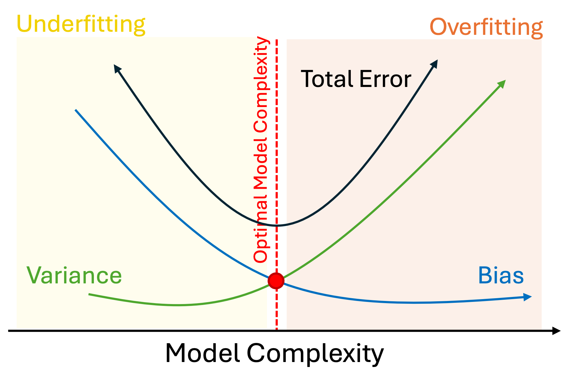
As mentioned earlier, overfitting occurs when a model has low bias but high variance. In contrast, underfitting refers to the situation wherein the model exhibits high bias and low variance. Figure 1 shows the bias-variance trade-off diagram [1].

Methods to Address

There are different methods and techniques to overcome both overfitting and underfitting. In the rest, we review some of them. Before reviewing the corresponding methods, we discuss two important techniques, namely regularization and cross validation, in details [1, 2].

Regularization

Regularization methods, such as L1-norm and L2-norm, mitigate the overfitting by adding a penalty term to the weights during updating [2].

The L1-norm, also known as Least Absolute Shrinkage and Selection Operator (Lasso) regression, introduces the absolute value of the coefficient magnitudes as a penalty term to the loss function \(\mathcal{L}\). Formally, it is defined as [2]

\[ \mathcal{L}_{L1} = \mathcal{L} + \lambda\sum_{i}^{M}|w_{i}| = \frac{1}{N}\sum_{i=1}^{N}(y_{i} - \hat{y}_{i})^{2} + \lambda\sum_{i}^{M}|w_{i}|, \]

where \(N\) and \(M\) are total number of samples and features, respectively; \(\lambda\) is the regularization parameter; \(w\) shows the weight (or coefficient); and \(y_{i}\) and \(\hat{y}_{i}\) represent the actual and predicted values, respectively. The L1 penalty encourages sparsity by shrinking less important weights toward zero that allows only the most significant features to contribute to the model during training [2].

The L2-norm, also known as Ridge regression or Euclidean norm, adds the square of the coefficient magnitudes as a penalty term to the loss function \(\mathcal{L}\). Formally, it is defined as [2]

\[ \mathcal{L}_{L1} = \mathcal{L} + \lambda\sum_{i}^{M}w_{i}^{2} = \frac{1}{N}\sum_{i=1}^{N}(y_{i} - \hat{y}_{i})^{2} + \lambda\sum_{i}^{M}w_{i}^{2} \]

Unlike L1 regularization, which enforces sparsity by driving some coefficients exactly to zero, L2 regularization uniformly penalizes large weights, leading to smaller but nonzero coefficients. This helps prevent overfitting by reducing model complexity while maintaining all features' contributions. However, it is highly sensitive to outliers in the data. Any outlier in the data can increase the error. To minimize this large penalty, the model will shift its parameters toward the outlier. Thus, the model is vulnerable to an improper fitting [2].

In summary, L1 and L2 regularization each offer distinct advantages depending on the characteristics of the data and the model. L1 regularization encourages sparsity by driving less important coefficients exactly to zero that makes it useful for feature selection in high-dimensional datasets. L2 regularization, on the other hand, penalizes large weights more smoothly that yields smaller but nonzero coefficients and promoting weight stability across correlated features. To leverage the benefits of both methods, Elastic Net regularization combines the L1 and L2 penalties as follows [2].

\[ \mathcal{L}_{ElasticNet} = \mathcal{L} + \lambda_{1}\sum_{i}^{M}|w_{i}| + \lambda_{2}\sum_{i}^{M}w_{i}^{2}, \]

where \(\lambda_{1}\) and \(\lambda_{2}\) control the contribution of the L1 and L2 terms, respectively. Elastic Net is particularly effective when dealing with datasets that contain highly correlated features or when both feature selection and regularization are desired simultaneously [2].

Cross-Validation

Cross-validation is a widely used technique to mitigate overfitting by providing a more reliable estimate of a model's generalization performance. The most common type is k-fold cross-validation, where the training dataset is divided into \(k\) equal-sized subsets, known as folds [3].

The training procedure is repeated \(k\) times. In each iteration, one fold is used as the validation set, while the remaining \((k - 1)\) folds are combined to form the training set. This ensures that every data point is used for both training and validation exactly once. Importantly, each iteration is independent, and the model learns separate weights corresponding to that iteration [3].

After completing all \(k\) iterations, the validation results from each fold are averaged to obtain the final performance estimate. This approach effectively reduces both bias and variance, thereby improving the model's ability to generalize and preventing overfitting [3].

Alleviate Underfitting and Overfitting

• Underfitting: To cope with the underfitting problem [1]:

  • Increase the model complexity: More complex models are able to learn underlying pattern of data. One efficient way is to use complex model (such as deep neural network models) rather than simpler model (such as linear/logistic regression) [1].

  • Add more features: Increasing the dimensionality of data, in terms of features, can help models to learn more complex patterns. Add more relevant features using feature engineering process [1].

  • Reduce regularization: Regularization techniques, such as the L1-norm (Lasso) and L2-norm (Ridge or Euclidean norm), play a crucial role in preventing overfitting by penalizing overly complex models. However, excessive regularization can lead to underfitting, as the model becomes too constrained to capture important patterns in the data. To mitigate this issue, the regularization strength can be reduced by using a smaller penalty coefficient [1].

  • Increase training duration: Increasing the number of epochs for training the model, let the model to learn more effectively [1].

• Overfitting:To prevent the model from overfitting [1]:

  • Increase training data: Increasing the dimensionality of training data, in terms of the number of samples, can help mitigate the overfitting problem. With more data, the model has greater opportunity to generalize and learn the underlying patterns, rather than memorizing the training examples [1].

  • Reduce model's complexity: Sometimes, the underlying data patterns are simple enough to be effectively learned by simpler models rather than highly complex ones. Complex models are not always the optimal choice; they tend to perform well only when the data are intricate and involve a large number of features, making pattern learning more challenging. To reduce the risk of overfitting in such cases, it is advisable to use simpler algorithms or architectures, decrease the number of layers, or reduce the number of neurons in the model [1].

  • Use regularization: Regularization techniques, such as the L1-norm (Lasso) and L2-norm (Ridge or Euclidean norm), play a crucial role in preventing overfitting by penalizing overly complex models [1].

  • Use dropout: Dropout is a regularization technique in neural networks that involves randomly deactivating a subset of neurons during training. This prevents the model from becoming overly reliant on specific neurons or pathways, thereby improving its ability to generalize to unseen data [1].

  • Implement early stopping: Early stopping is a regularization technique that halts training when the model's performance on a separate validation set begins to deteriorate, even if its performance on the training set continues to improve. This approach helps prevent overfitting by stopping the learning process before the model starts to memorize noise in the training data [1].

  • Perform feature selection: Irrelevant or redundant features can cause the model to overfit to noise. Removing those features improves generalization and the model's performance [1].

  • Deploy data augmentation: When the diversity of a dataset is low, a model is more likely to memorize the data patterns rather than learning them. Data augmentation is a technique that addresses this issue by increasing dataset diversity. To this end, it generates new data points through transformations of existing samples [1].

  • Apply cross-validation: Cross-validation guarantees that every data point in the training set is used for both training and validation exactly once. Therefore, it avoids the model to be trained over fixed sets. As a result, both bias and variance are decreased [1].

Vanishing and Exploding Gradient

Gradients are the key parameters in model training. During backpropagation in neural network (NN) models, the gradient of the loss is computed w.r.t. the weights and biases separately. Then, based on the optimization algorithm, such as Stochastic Gradient Descent (SGD) or Adaptive Moment Estimation (Adam)-both driven by the gradient descent mechanism, the weights and biases are updated layer by layer. This implies that in each layer, the weights are multiplied recursively by gradient-based updates so that the overall loss is minimized across the network. However, if these multipliers become excessively small or large, the learning process encounters major difficulties. The former issue is referred to as gradient vanishing, while the latter is known as gradient exploding [4].

Gradient Vanishing

One common challenge in neural networks, particularly recurrent neural networks (RNNs), that often leads to underfitting is \textbf{gradient vanishing}. During backpropagation, if the gradients are repeatedly multiplied by values smaller than one, they shrink exponentially as they propagate backward through the layers. Consequently, the weights in the early layers approach zero, preventing the model from learning useful patterns. This phenomenon results in slow or completely stalled learning [4].

Gradient Exploding

The opposite of gradient vanishing is the gradient exploding problem. It occurs when the gradients grow exponentially during backpropagation—often in deep or recurrent networks. This causes the model parameters to oscillate or diverge. When gradient exploding happens, the loss fails to converge, and the model parameters may take extremely large values that results in unstable training or numerical overflow. Gradient exploding typically arises when [4]:

• The network is very deep, and the product of large gradients across multiple layers accumulates exponentially [4].

• Improper weight initialization leads to excessively large parameter updates [4].

• The learning rate is too high that amplifies each weight update [4].

Techniques to Cope with Gradient Vanishing and Exploding

Before diving into the gradient vanishing and exploding problems, it is essential to review several fundamental techniques that can effectively alleviate both issues.

Weight Initialization

Avoiding random initialization of weights and adopting principled initialization strategies can significantly reduce the probability of both vanishing and exploding gradients. Techniques such as Kaiming initialization and Xavier initialization set the initial weights at appropriate scales, thereby maintaining stable gradient propagation during early training [5, 6].

• Kaiming Initialization: Kaiming (or He) initialization is suitable for layers that use the ReLU activation function. It prevents vanishing gradients by assigning a larger variance to the initial weights. There are two common variants [5]:

  • Kaiming Normal Initialization: Weights are drawn from a normal distribution with a mean of 0 and a standard deviation of \(\sqrt{\frac{2}{n_{in}}}\):

    \[ w_i \sim \mathcal{N}(0, \sqrt{\tfrac{2}{n_{in}}}), \]

    where \(n_{in}\) is the number of input units to the layer.

  • Kaiming Uniform Initialization: Weights are drawn from a uniform distribution in the range:

    \[ w_i \sim U\left(-\sqrt{\tfrac{6}{n_{in}}}, \sqrt{\tfrac{6}{n_{in}}}\right), \]

    that ensures variance preservation across layers.

• Xavier Initialization: Xavier (or Glorot) initialization is more suitable for layers using Sigmoid or Tanh activation functions. It aims to keep the variance of activations and gradients consistent across layers. Two variants exist [6]:

  • Normal Xavier Initialization: Weights are drawn from a normal distribution with a mean of 0 and a standard deviation of \(\sqrt{\frac{2}{n_{in} + n_{out}}}\):

    \[ w_i \sim \mathcal{N}\left(0, \sqrt{\tfrac{2}{n_{in} + n_{out}}}\right), \]

    where \(n_{in}\) and \(n_{out}\) denote the number of input and output units, respectively.

  • Uniform Xavier Initialization: Weights are drawn from a uniform distribution in the range:

    \[ w_i \sim U\left(-\sqrt{\tfrac{6}{n_{in} + n_{out}}}, \sqrt{\tfrac{6}{n_{in} + n_{out}}}\right) \]

Normalization

Normalizing inputs to each layer stabilizes gradient flow, accelerates convergence, and mitigates both vanishing and exploding gradients. Two widely used normalization methods are described below.

• Batch Normalization: batch, ensuring zero mean and unit variance. Consequently, the input to each layer becomes dependent on the batch statistics. Although highly effective for large batch sizes, it can be less stable for small batches or recurrent neural networks (RNNs), where batch statistics fluctuate significantly [7].

• Layer Normalization: This approach normalizes activations across the features of each individual sample, independently of other samples in the batch. This makes it particularly suitable for small or variable batch sizes, as in RNNs and natural language processing tasks [8].

Additional Strategies for Gradient Stabilization

Several other strategies can further mitigate the vanishing and exploding gradient problems [4].

• Alternative Activation Functions: Saturating activation functions such as Sigmoid and Tanh are prone to vanishing gradients because their derivatives approach zero for large input magnitudes. In contrast, ReLU maintains gradients close to 1 for positive inputs, preventing exponential shrinkage [4].

• Residual and Skip Connections: Architectures such as ResNets incorporate shortcut connections that allow gradients to bypass intermediate layers, ensuring more effective propagation to earlier layers [4].

• Gradient Clipping: This widely used technique constrains the gradient norm to a predefined threshold (e.g., by rescaling gradients when their magnitude exceeds a limit), thereby preventing instability due to gradient explosion [4].

• Learning Rate Adjustment: A smaller learning rate ensures smoother parameter updates, helping avoid overshooting and gradient amplification during optimization [4].

• Gated Architectures (for RNNs): In sequential models, gating mechanisms such as those in Long Short-Term Memory (LSTM) regulate information and gradient flow over time, effectively mitigating both vanishing and exploding gradients in long sequences [4].

In practice, both vanishing and exploding gradients can coexist in different parts of a deep network. Therefore, combining techniques such as careful initialization, normalization, skip connections, and adaptive optimizers (e.g., Adam) is essential to achieve stable and efficient training.

References

[1] GeeksforGeeks, “Bias and variance in machine learning,” GeeksforGeeks, accessed: July 12, 2025, https://www.geeksforgeeks.org/machine-learning/bias-vs-variance-in-machine-learning/.

[2] GeeksforGeeks, “Regularization in machine learning,” GeeksforGeeks, accessed: September 18, 2025, https://www.geeksforgeeks.org/machine-learning/regularization-in-machine-learning/.

[3] GeeksforGeeks, “Cross Validation in Machine Learning,” GeeksforGeeks, accessed: July 23, 2025, https://www.geeksforgeeks.org/machine-learning/cross-validation-machine-learning/.

[4] GeeksforGeeks, “Vanishing and exploding gradients problems in deep learning,” GeeksforGeeks, accessed: July 23, 2025, https://www.geeksforgeeks.org/deep-learning/vanishing-and-exploding-gradients-problems-in-deep-learning/.

[5] GeeksforGeeks, “Kaiming initialization in deep learning,” GeeksforGeeks, accessed: July 23, 2025, https://www.geeksforgeeks.org/deep-learning/kaiming-initialization-in-deep-learning/.

[6] GeeksforGeeks, “Xavier initialization,” GeeksforGeeks, accessed: July 23, 2025, https://www.geeksforgeeks.org/deep-learning/xavier-initialization/.

[7] GeeksforGeeks, “What is batch normalization in deep learning?,” GeeksforGeeks, accessed: July 23, 2025, https://www.geeksforgeeks.org/deep-learning/what-is-batch-normalization-in-deep-learning/.

[8] GeeksforGeeks, “What is layer normalization?,” GeeksforGeeks, accessed: July 23, 2025, https://www.geeksforgeeks.org/deep-learning/what-is-layer-normalization/.