Evaluation Metrics

After training (or tuning/fitting) a classification model, it is important to evaluate its performance and assess how well it can make predictions. To do this, the model is provided with test data, i.e., unseen data that were not used during training, and its performance is measured using various evaluation metrics. Depending on the type of the ML model, various evaluation metrics are employed.

Classification

Several metrics can be used to evaluate the performance of a tuned model for classification purposes (binary classification). In this chapter, we focus on key metrics: Accuracy, Recall (or true positive rate), false positive rate, Precision, F1-score, and ROC-AUC.

Confusion Matrix

Before discussing evaluation metrics, it is important to understand the confusion matrix and its components, which play a crucial role in model evaluation [1].

A confusion matrix consists of four elements: true positive (TP), false positive (FP), true negative (TN), and false negative (FN). Figure 1 illustrates the confusion matrix, where columns represent the actual values and rows represent the predicted values. TP and TN occur when the model's predictions match the actual values. Conversely, if the model predicts a negative (positive) instance as positive (negative), it corresponds to FP (FN) [1].

Accuracy

Accuracy indicates how accurate a model is to predict both positive and negative classes correctly [1].

\[ \text{Accuracy} = \frac{\text{TP} + \text{TN}}{\text{TP} + \text{FP} + \text{TN} + \text{FN}} \]

Recall

Recall, also known as true positive rate (TPR), measures how effectively a model identifies positive instances. Specifically, it is the proportion of true positive instances relative to all actual positive samples, including both correctly predicted positives and positive instances that were incorrectly predicted as negative [1].

\[ \text{Recall} = \frac{\text{TP}}{\text{TP} + \text{FN}} \]

False Positive Rate (FPR)

The false positive rate (FPR) measures how often a model incorrectly classifies negative instances as positive. Specifically, it is the proportion of negative samples that are misclassified as positive relative to all actual negative samples [1].

\[ \text{FPR} = \frac{\text{FP}}{\text{TN} + \text{FP}} \]

Precision

Precision describes how precise a model is to classify true positive instances. Precision measures the proportion of true positive instances among all predicted positive instances [1].

\[ \text{Precision} = \frac{\text{TP}}{\text{TP} + \text{FP}} \]

F1-score

In imbalanced datasets, the arithmetic mean can be skewed by high values. In contrast, the harmonic mean gives more weight to lower values. The F1-score (that is F\(_{\beta}\)-score with \(\beta = 1\)) is the harmonic mean of precision and recall, that guarantees a low value in either metric results in a correspondingly low F1-score [1]

\[ \text{F1-score} = \frac{(1 + \beta^{2})\times\text{Precision}\times\text{Recall}}{\beta^{2}\times\text{Precision} + \text{Recall}} \overset{\beta = 1}{=} 2\times\frac{\text{Precision}\times\text{Recall}}{\text{Precision} + \text{Recall}} \]

ROC-AUC

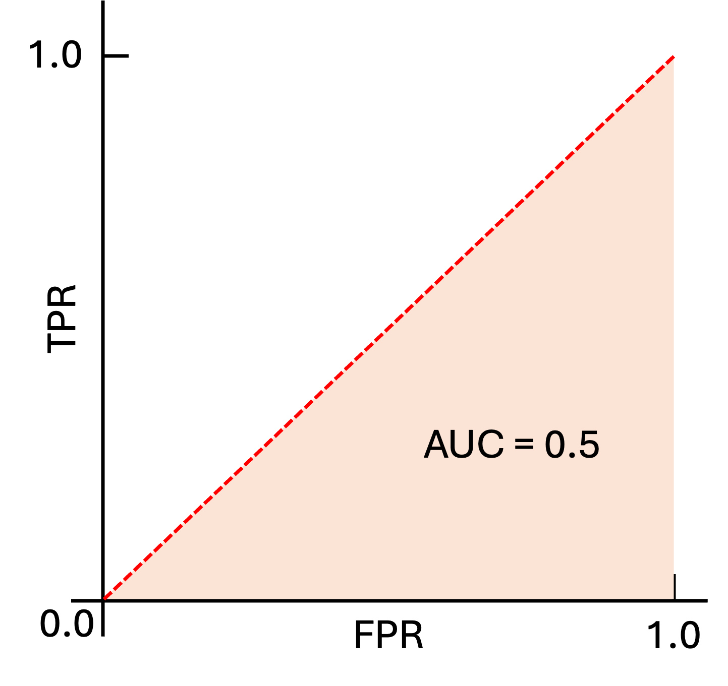
Accuracy depends on a specific decision threshold. In contrast, the Receiver Operating Characteristic (ROC) curve provides a visual representation of model performance across all thresholds, making it threshold-independent. The ROC plots the True Positive Rate (TPR) against the False Positive Rate (FPR). The Area Under the Curve (AUC) quantifies the probability that the model will assign a higher score to a randomly chosen positive instance than to a randomly chosen negative one [1].

Figure 2 illustrates the ROC curve for a binary classification scenario in which the model makes predictions completely at random, like a coin flip. In this case, the AUC equals 0.5 [1].

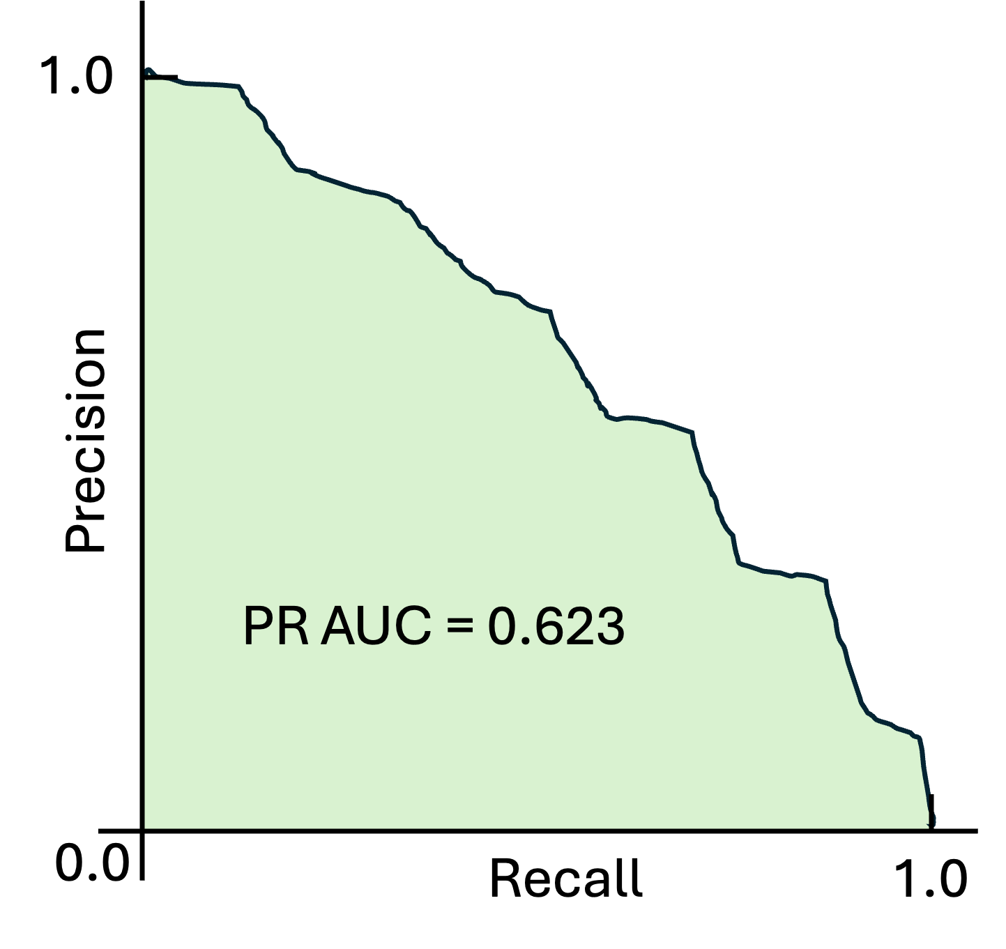
The ROC-AUC concept can be extended to Precision-Recall (PR) curves to more effectively evaluate model performance. Figure 3 shows the PR curve and its corresponding AUC for an example scenario, providing insight into how the model balances precision and recall. PR-AUC is particularly useful for imbalanced datasets, where the positive class is rare, because it focuses on the model's performance with respect to the minority class rather than being dominated by the majority class, as can happen with ROC-AUC. In general, higher PR-AUC values indicate better model performance [1].

Regression

Unlike classification models, which predict discrete classes or labels, regression models produce continuous numerical values as output. Therefore, specific evaluation metrics are needed to assess the performance of regression models.

In regression models, the key concept for evaluating performance is error (or residual). The error is defined as the difference between the actual value and the predicted value. Regression models are developed to minimize the error.

Mean Absolute Error (MAE)

Mean absolute error (MAE) measures the arithmetic mean of absolute errors for predictions [2].

\[ \text{MAE} = \frac{1}{N} \sum_{i=1}^{N} |\text{Actual}_i - \text{Predicted}_i| \]

MAE treats all errors equally, assigning the same weight to small and large errors. As a result, large errors are not penalized more heavily than small ones. This property also makes MAE relatively robust to outliers, i.e., extreme values that lie far from the typical range of the data. Overall, MAE is appropriate for balanced data [2].

Mean Squared Error (MSE)

Mean squared error (MSE) calculates the arithmetic mean of squared differences between the actual data and the predicted values [2].

\[ \text{MSE} = \frac{1}{N} \sum_{i=1}^{N} (\text{Actual}_i - \text{Predicted}_i)^2 \]

Squaring the errors makes the MSE enable to penalize larger errors more heavily than smaller errors, making it sensitive to outliers in the data [2].

Root Mean Squared Error (RMSE)

Root mean squared error (RMSE) measures to root of MSE, i.e., the arithmetic mean of squared differences between the actual data and the predicted values [2].

\[ \text{RMSE} = \sqrt{\text{MSE}} = \sqrt{\frac{1}{N}\sum_{i=1}^{N} (\text{Actual}_i - \text{Predicted}_i)^2} \]

R-squared Score

R-squared Score (R²-score) is a measure of goodness of fit, i.e., it measures how close the data points are to the fitted line [2].

\[ R^2\text{-score} = 1 - \frac{\text{SS}_{\text{RES}}}{\text{SS}_{\text{TOT}}} = 1 - \frac{\sum_{i=1}^{N}(y_i - \hat{y}_i)^2}{\sum_{i=1}^{N}(y_i - \bar{y})^2}, \]

where SSR_RES and SS_TOT show the sum of squares residuals (errors) and total, respectively. The former, measures the sum of squared difference between predicted values and actual values. The latter calculated the sum of squared difference between the actual values and their arithmetic mean [2].

Clustering

Unlike classification and regression problems, where data are labeled, clustering deals with unlabeled data. Since no ground-truth labels are available, clustering models group data based on similarities such as distance or distribution. As a result, traditional evaluation metrics used in classification or regression are not directly applicable to clustering.

Silhouette Score

The Silhouette Score evaluates the quality of clustering by measuring how well each data point fits within its assigned cluster compared to neighboring clusters. A score close to +1 indicates that a data point is well-matched to its own cluster and far from other clusters, while a score near 0 suggests that the point lies on or near a cluster boundary. Negative scores (close to –1) indicate that a data point may have been misassigned to the wrong cluster. The overall clustering quality is typically assessed by the average silhouette score across all data points, with higher values reflecting better-defined and more clearly separated clusters [3].

\[ s(i) = \frac{b(i) - a(i)}{\max\{a(i), b(i)\}}, \]

where \(a(i)\) is the inter-cluster distance, i.e., average distance from point \(i\) to all other points in the same cluster; and \(b(i)\) represents the nearest-cluster distance, i.e., minimum average distance from point \(i\) to points in the nearest neighboring cluster [3].

Davies-Bouldin Index

The Davies-Bouldin Index (DBI) is an internal evaluation metric that measures the quality of clustering based on the trade-off between cluster compactness and separation. Compactness is quantified by the average distance of data points within a cluster to their centroid, while separation is measured by the distance between cluster centroids. A lower DBI value indicates better clustering, as it reflects more compact clusters that are well separated from each other. Since DBI relies only on the data and cluster assignments, it does not require external ground-truth labels [3].

\[ DBI = \frac{1}{k} \sum_{i=1}^{k} \max_{i \neq j} \left( \frac{S_i + S_j}{M_{ij}} \right), \]

where \(k\) is the number of clusters; \(S_{i}\) represents the compactness of the cluster \(i\), that is, the average distance of all points of the cluster \(i\) to its centroid; and \(M_{i}\) indicates the separation between the clusters, that is, the distance between the centroids of the clusters \(i\) and \(j\). Notably, \((S_{i} + S_{j}) / M_{ij}\) compares the similarity between clusters \(i\) and \(j\) [3].

Ranking and Recommendation

In ranking and recommendation tasks, the developed machine learning system generates a list of outputs ranked from highest to lowest relevance. However, according to the ground-truth data, some truly relevant items may be incorrectly classified as irrelevant. Evaluation metrics such as Recall@k, Precision@k, and Mean Average Precision (mAP) are commonly used to assess the model's performance in capturing and ranking the relevant results accurately.

Precision@K

In ranking and recommendation tasks, the evaluation is typically limited to the top-K retrieved items. In this context, Precision@K measures how many of the items within the top-K positions are relevant. Formally, Precision@K is defined as the ratio of relevant items retrieved in the top-K results to K. Therefore, we have [4].

\[ \text{Precision@K} = \frac{\text{TP}}{\text{TP} + \text{FP}} \]

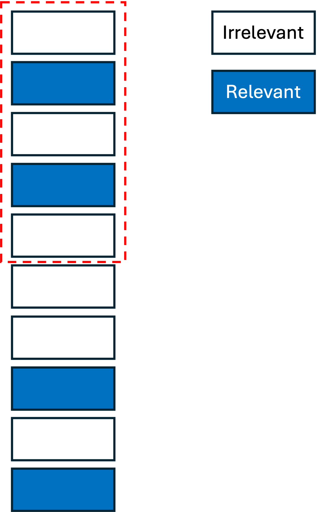
Figure 4 illustrates an example of a ranking system with K \( = 5\). As shown, the model successfully identifies two relevant items out of four total relevant items within the top-K results. Therefore, the Precision@K value is computed as \(2 / 5 = 0.4\).

It is worth noting that Precision@K is highly sensitive to the choice of K. Consider a case where only two relevant items exist in the ground-truth data, and the model successfully retrieves both within the top-K results. If K is set to a large value, the precision will decrease substantially, since the number of retrieved items increases while the number of relevant items remains constant.

Recall@K

Recall is defined as the model's ability to identify true positive instances in its predictions. In ranking and recommendation tasks, Recall@K measures how many of the relevant items are correctly retrieved by the model within the top-K positions. Formally, Recall@K is defined as the ratio of relevant items retrieved in the top-K results to the total number of relevant items in the ground-truth data. Therefore, we have [4]

\[ \text{Recall@K} = \frac{\text{TP}}{\text{TP} + \text{FN}} \]

Referring to the example provided in Fig. 4, the Recall@K value is computed as \(2 / 4 = 0.5\). Therefore, Recall@K reduces the sensitivity to K observed in Precision@K. However, although Recall@K is less sensitive to the value of K compared to Precision@K, it is insensitive to the relative ranking of relevant items within the top-K positions. For example, consider a case where only two relevant items exist in the ground-truth data, and both are retrieved within the top-K results but appear at lower ranks (e.g., positions 9 and 10 when K \(= 10\)). In this case, Recall@K equals 1.0, even though the ranking quality is poor.

Mean Reciprocal Rank@K (MRR@K)

To understand Mean Reciprocal Rank@K (MRR@K), it is necessary to introduce Reciprocal Rank@K (RR@K) first. RR@K is a metric that focuses on the position of the first relevant item within the top-K results. It is defined as [4].

\[ \text{RR} = \frac{1}{\text{Rank of the first relevant item}} \]

For example, considering the example in Fig. 4, the RR@K is given as \(1 / 2 = 0.5\). Considering \(U\) ranked lists in the results, each corresponding to a query in an information retrieval task or a user in a recommendation system, MRR@K is defined as the average of RR@K across all \(U\) lists, i.e.,

\[ \text{MRR@K} = \frac{1}{U} \sum_{u=1}^{U} RR@K_u \]

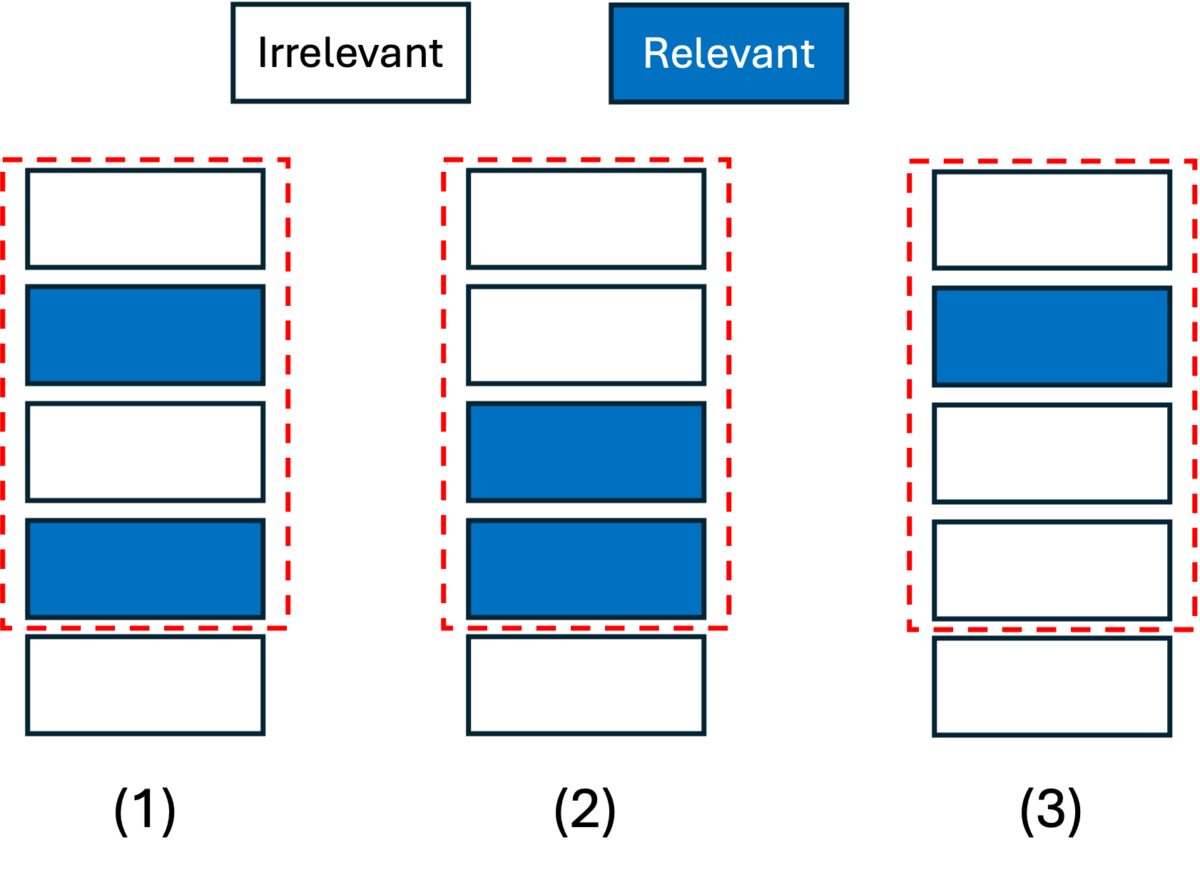
For instance, Fig. 5 illustrates a ranking system with three lists in the outputs. As shown, the positions of the first relevant items are 2, 3, and 2 in the first, the second, and the third lists, respectively. Therefore, the corresponding RR@K values are computed as \(1 / 2 = 0.5\), \(1 / 3 = 0.33\), and \(1 / 2 = 0.5\). Accordingly, the MRR@K is equal to \((0.5 + 0.33 + 0.5) / 3 = 0.44\).

MRR@K addresses the limitation of Precision@K and Recall@K, both of which ignore the ranks of relevant items within the top-K results. However, MRR@K only accounts for the rank of the first relevant item and disregards the positions of other relevant items that may also appear within the top-K list.

Mean Average Precision@K (mAP@K)

Unlike MMR@K that measures the rank of the first relevant item in the output lists, Mean Average Precision@K (mAP@K) considers all relevant elements in the top-K positions. mAP@K is the mean of AP@K values. Taking into account \(N_{u}\) relevant items in the list \(u\), we have [4]

\[ \text{AP@K}_u = \frac{1}{N_u} \sum_{k=1}^{K} \text{Precision}(k) \cdot \text{rel}(k), \]

where Precision\((k)\) is the precision of predictions at top-\(k\) positions, where \(k = 1, \dots, K\); also, rel\((k)\) is the relevance score of the item, that can be a binary value (relevant/not relevant) or a graded score (e.g., 0, 1, 2, 3). In the case of AP@K, we defined is as a binary variable where is equal to 1 if the item is relevant, and 0 otherwise. For example, referring to Fig. 5, for \(u = 1\), we have:

• \(k = 1\): Precision\((k) = 0 / 1 = 0\), rel\((k) = 0\)

• \(k = 2\): Precision\((k) = 1 / 2 = 0.5\), rel\((k) = 1\)

• \(k = 3\): Precision\((k) = 1 / 3 = 0.33\), rel\((k) = 0\)

• \(k = 4\): Precision\((k) = 2 / 4 = 0.5\), rel\((k) = 1\)

Therefore

\[ \text{AP@K}_{1}= \frac{0\times 0 + 0.5\times 1 + 0.33\times 0 + 0.5\times 1}{2} = \frac{0 + 0.5 + 0 + 0.5}{2} = \frac{1.0}{2} = 0.5 \]

Accordingly, for \(u = 2\) and \(u = 3\), we have

\[ \text{AP@K}_{2}= \frac{0\times 0 + 0\times 0 + 0.33\times 1 + 0.0.5\times 1}{2} = \frac{0 + 0 + 0.33 + 0.5}{2} = \frac{0.83}{2} = 0.42 \]

\[ \text{AP@K}_{3}= \frac{0\times 0 + 0.5\times 1 + 0\times 0 + 0\times 0}{1} = \frac{0 + 0.5 + 0 + 0}{1} = \frac{0.5}{1} = 0.5 \]

mAP@K measure the mean of all AP@K values as

\[ \text{mAP@K} = \frac{1}{U} \sum_{u=1}^{U} \text{AP@K}_u \]

Therefore, mAP@K value for the above-mentioned example in Fig. 5 is computed as

\[ \text{mAP@K}= \frac{0.5 + 0.42 + 0.5}{3} = \frac{1.42}{3} = 0.47 \]

Normalized Discounted Cumulative Gain@K (nDCG@K)

It is important not only to determine whether an item is relevant within an output list but also to evaluate how relevant it is. None of the aforementioned metrics account for the degree of relevance of items. In contrast, Normalized Discounted Cumulative Gain@K (nDCG@K) captures this aspect by assigning graded relevance scores to items. To compute nDCG@K, the Discounted Cumulative Gain@K (DCG@K) is first calculated, which applies a logarithmic discount factor based on the position of each item in the ranked list, i.e., \(\log_{2}(i + 1)\). Formally, DCG@K is defined as [4]

\[ \text{DCG@K} = \sum_{i=1}^{K} \frac{\text{rel}_i}{\log_2(i+1)} \]

In addition to the predicted ranks, the Ideal DCG (IDCG) metric represents the maximum possible DCG for a given set of results. nDCG@K normalizes the DCG with respect to the IDCG, yielding a score between 0 and 1. Formally [4],

\[ \text{nDCG@K} = \frac{\text{DCG@K}}{\text{IDCG@K}} \]

For instance, consider the results in Fig. 6. There are three output lists, labeled 1, 2, and 3, and an ideal list with the ideal ranking of the items.

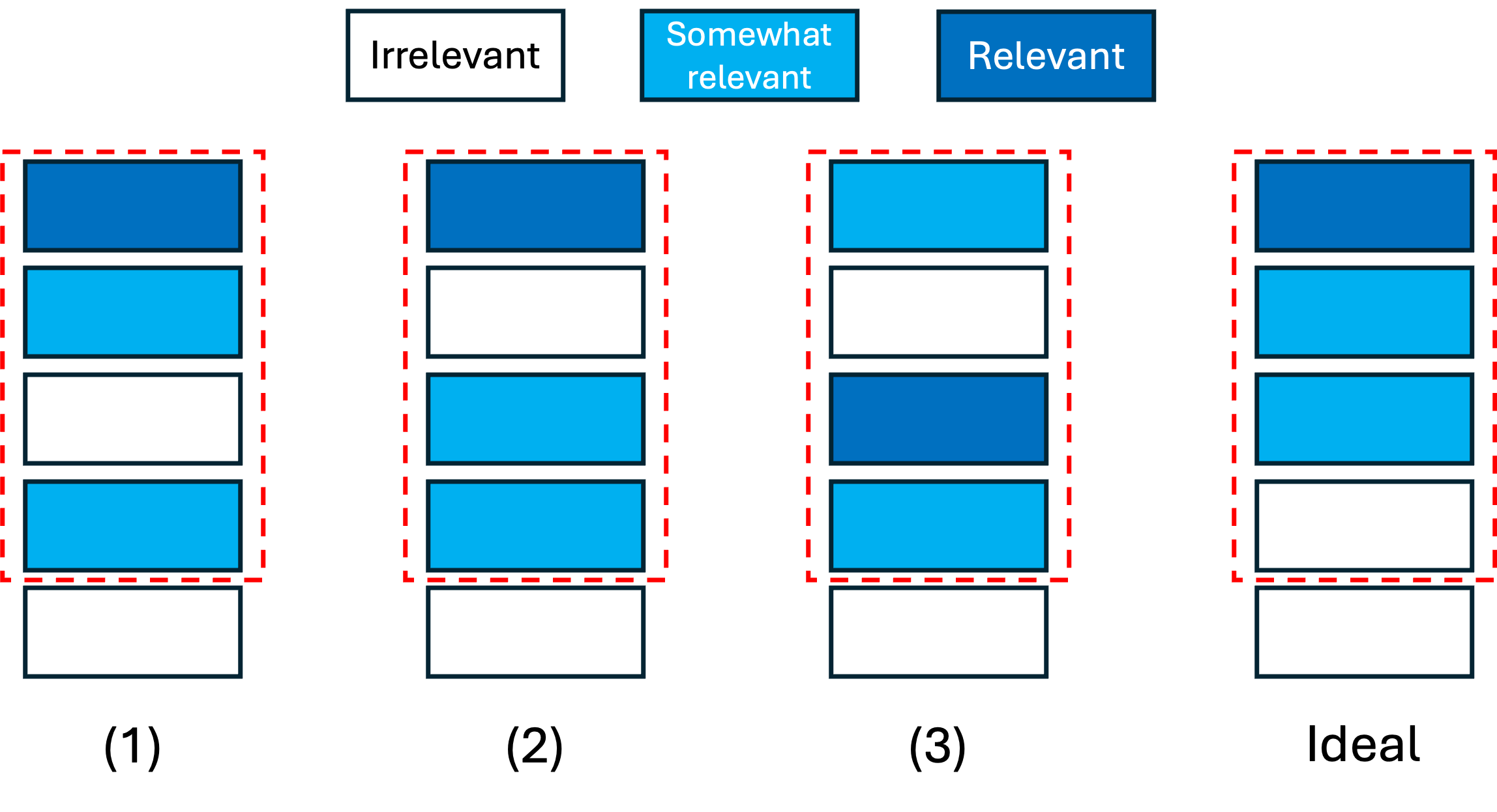
Since the items are categorized as irrelevant, somewhat relevant, and relevant, we define relevance scores 0, 1, and 2, respectively. Therefore, for each list \(u\), the corresponding DCG@K\(_{u}\) is computed as

\[ \text{DCG@K}_{1} = \frac{2}{\log_{2}(1+1)} + \frac{1}{\log_{2}(2+1)} + \frac{0}{\log_{2}(3+1)} + \frac{1}{\log_{2}(4+1)} = \frac{2}{1} + \frac{1}{1.59} + 0 + \frac{1}{2.32} = 2 + 0.63 + 0.43 = 3.06 \]

\[ \text{DCG@K}_{2} = \frac{2}{\log_{2}(1+1)} + \frac{0}{\log_{2}(2+1)} + \frac{1}{\log_{2}(3+1)} + \frac{1}{\log_{2}(4+1)} = \frac{2}{1} + 0 + \frac{1}{2} + \frac{1}{2.32} = 2 + 0.5 + 0.43 = 2.93 \]

\[ \text{DCG@K}_{2} = \frac{1}{\log_{2}(1+1)} + \frac{0}{\log_{2}(2+1)} + \frac{2}{\log_{2}(3+1)} + \frac{1}{\log_{2}(4+1)} = \frac{1}{1} + 0 + \frac{2}{2} + \frac{1}{2.32} = 1 + 1 + 0.43 = 2.43 \]

Also, IDCG@K value is given by

\[ \text{IDCG@K} = \frac{2}{\log_{2}(1+1)} + \frac{1}{\log_{2}(2+1)} + \frac{1}{\log_{2}(3+1)} + \frac{0}{\log_{2}(4+1)} = \frac{2}{1} + \frac{1}{1.59} + \frac{1}{2} + 0 = 2 + 0.63 + 0.5 = 3.13 \]

Accordingly, the nDCG@K for each list is calculated as

\[ \text{nDCG@K}_{1} = \frac{\text{DCG@K}_{1}}{\text{IDCG@K}} = \frac{3.06}{3.13} = 0.98 \]

\[ \text{nDCG@K}_{2} = \frac{\text{DCG@K}_{2}}{\text{IDCG@K}} = \frac{2.93}{3.13} = 0.94 \]

\[ \text{nDCG@K}_{3} = \frac{\text{DCG@K}_{3}}{\text{IDCG@K}} = \frac{2.43}{3.13} = 0.78 \]

References

[1] Google, “Ml concepts - crash course,” Google, accessed: 2025, https://developers.google.com/machine-learning/crash-course/prereqs-and-prework.

[2] E. Lewinson, “A comprehensive overview of regression evaluation metrics,” Nvidia, accessed: April 20, 2023, https://developer.nvidia.com/blog/a-comprehensive-overview-of-regression-evaluation-metrics/.

[3] GeeksforGeeks, “Evaluation metrics for search and recommendation systems,” GeeksforGeeks, accessed: July 23, 2025, https://www.geeksforgeeks.org/machine-learning/clustering-metrics/.

[4] L. Monigatti, “Clustering metrics in machine learning,” Weaviate, accessed: May 28, 2024, https://weaviate.io/blog/retrieval-evaluation-metrics.