Recurrent Neural Network

Recurrent Neural Networks (RNNs) are time-dependent architectures in which outputs from previous time steps participate in the prediction of the current output. Unlike MLPs and CNNs, which apply traditional backpropagation, RNNs employ Backpropagation Through Time (BPTT), a variant designed to handle temporal dependencies. BPTT follows the same fundamental procedure as standard backpropagation, i.e., calculating errors from the output layer back to the input; yet, it propagates the sum of errors over all time steps that allows the network to learn from sequential dependencies. Figure 1 illustrates the conceptual difference between an MLP and an RNN [1].

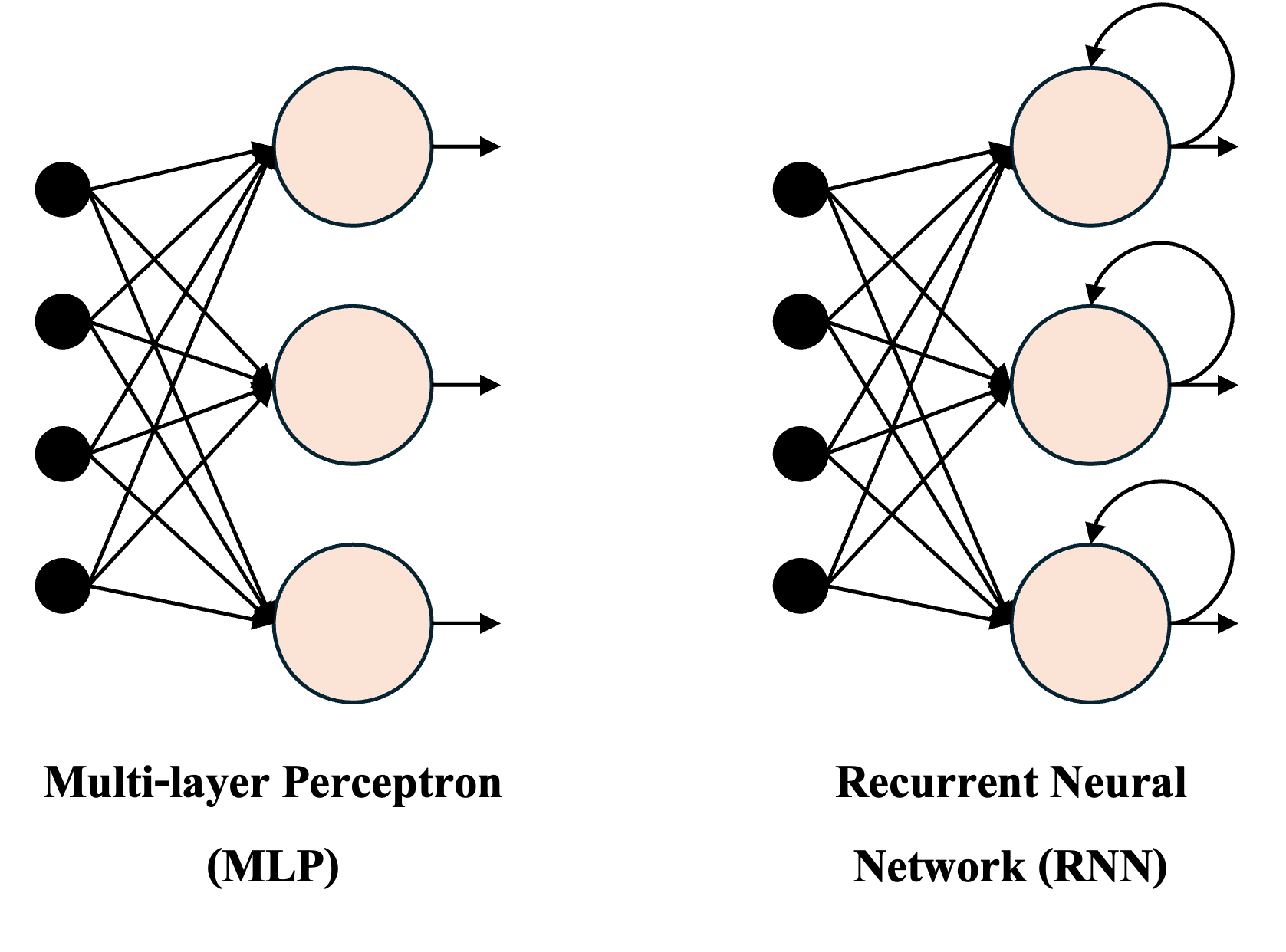
Figure 2 depicts the basic computational structure of an RNN unfolded across multiple time steps. At each time step \(t\), the model takes as input the current feature vector \(x_{t}\), the hidden state from the previous time step \(h_{t-1}\), and produces both an updated hidden state \(h_{t}\) and an output \(o_{t}\) [2].

The hidden state acts as the network's internal memory that carries temporal information across time. The hidden state at time step \(t\) is computed as [2]:

\[ h_{t} = \tanh(U x_{t} + V h_{t-1} + b_h), \]

where \(U\) is the weight matrix associated with the input \(x_{t}\), \(V\) shows the weight matrix associated with the previous hidden state \(h_{t-1}\), and \(b_{h}\) represents bias term for the hidden layer.

Notabely, the RNN shares the same weights (\(U\), \(W\), and \(b_{h}\)) across all time steps, meaning that these parameters are time-invariant. This parameter sharing reduces model complexity and ensures consistent learning across temporal contexts [2].

Once the hidden state \(h_{t}\) is computed, the output at time \(t\) is generated using an activation function, commonly the sigmoid function \(\sigma(\cdot)\) [2]:

\[ o_{t} = \sigma(W_{o} h_{t} + b_{o}), \]

where \(W\) and \(b_{o}\) denote the output-layer weights and bias, respectively. The term \(o_{t}\) represents the model's external output (used for tasks such as text generation, translation, or forecasting), while \(h_{t}\) serves as the internal output passed to the next time step \((t + 1)\) [2].

The RNN architecture offers both advantages and disadvantages [2]:

• Advantages:

  • Can handle variable-length sequential inputs.

  • Maintains internal memory (hidden states) that captures temporal dependencies.

  • Shares parameters across time, reducing model size and complexity.

  • Well-suited for sequence-based tasks such as language modeling, translation, speech recognition, and text summarization.

• Disadvantages:

  • Prone to the vanishing and exploding gradient problems during training.

  • Struggles with long-term dependencies, making it less effective for tasks requiring long-range context.

  • Sequential computation limits parallelization, leading to slower training compared to feed-forward architectures.

Long Short-Term Memory

As mentioned earlier, RNNs are prone to the gradient vanishing problem. The Long Short-Term Memory (LSTM) architecture addresses this issue by introducing a long-term memory mechanism (see Fig. 3) [3-5].

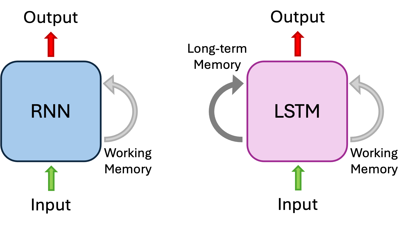
LSTMs maintain both short-term and long-term states across time steps. Figure 4 illustrates the architecture of an LSTM, which consists of three gates: forget gate, input gate, and output gate [4].

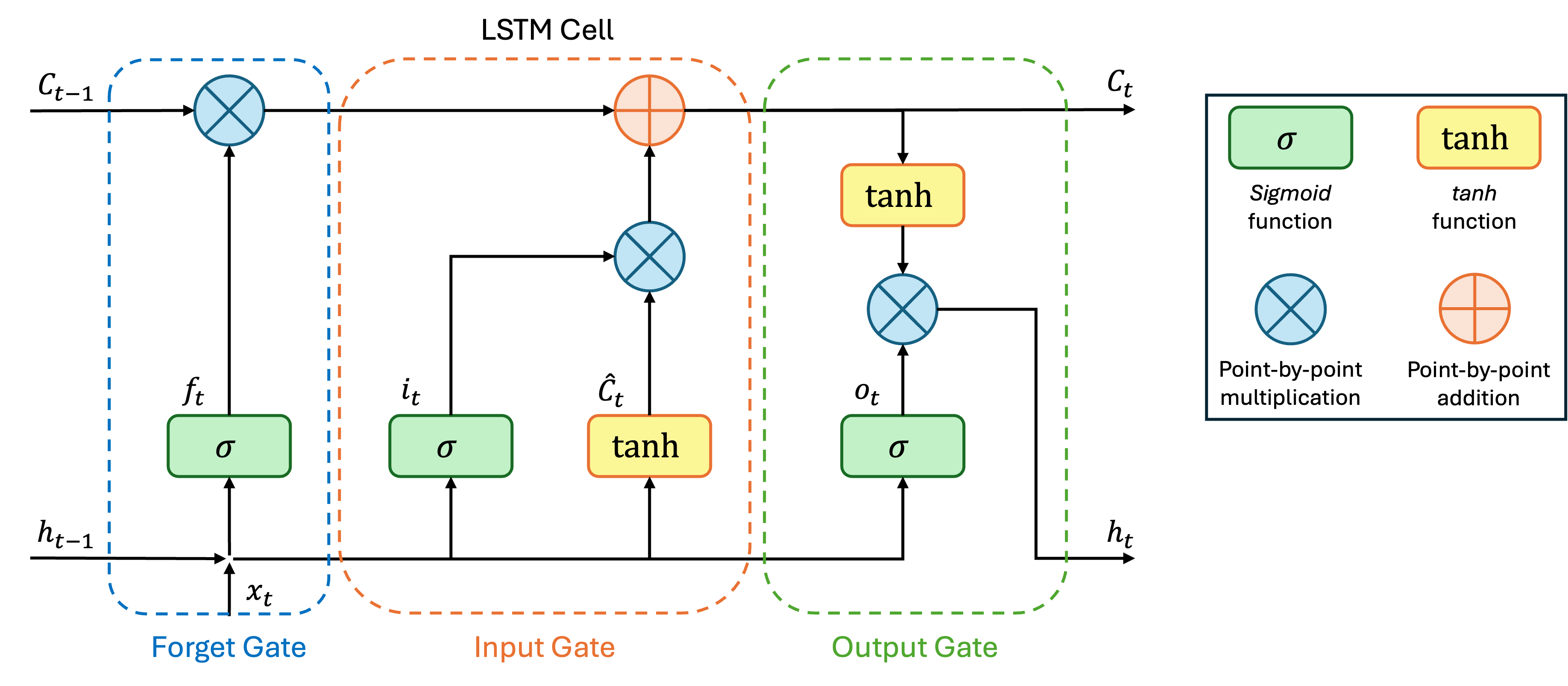
The forget gate allows the model to selectively discard irrelevant information from the past. Specifically, the previous hidden state, \(h_{t-1}\), and the current input, \(x_{t}\), are processed to generate a forget vector, \(f_{t}\), that controls how much of the previous cell state \(C_{t-1}\) should be retained [4]:

\[ f_{t} = \sigma\Big(W_{f} \cdot [h_{t-1}, x_{t}] + b_{f}\Big), \]

where \(W_{f}\) and \(b_{f}\) represent the weights and bias of the forget gate, respectively. The updated cell state is then partially preserved as \(C_{t-1} \odot f_{t}\) [4].

The input gate determines what new information should be added to the cell state. Both \(h_{t-1}\) and \(x_{t}\) are passed through a sigmoid layer and a \(\tanh\) layer to generate candidate updates [4]:

\[ \begin{split} i_{t} &= \sigma\Big(W_{i} \cdot [h_{t-1}, x_{t}] + b_{i}\Big),\\ \hat{C}_{t} &= \tanh\Big(W_{c} \cdot [h_{t-1}, x_{t}] + b_{c}\Big), \end{split} \]

where \(i_{t}\) represents the input modulation gate, and \(\hat{C}_{t}\) represents the candidate cell state. The new cell state \(C_{t}\) is then updated as follows [4]:

\[ C_{t} = f_{t} \odot C_{t-1} + i_{t} \odot \hat{C}_{t} \]

Finally, the output gate controls what part of the cell state should be output at each time step. The gate first computes an activation \(o_{t}\), then multiplies it with the \(\tanh\)-transformed cell state to obtain the new hidden state \(h_{t}\) [4]:

\[ \begin{split} o_{t} &= \sigma\Big(W_{o} \cdot [h_{t-1}, x_{t}] + b_{o}\Big),\\ h_{t} &= o_{t} \odot \tanh(C_{t}), \end{split} \]

where \(W_{o}\) and \(b_{o}\) denote the weights and bias terms for the output gate. In summary, LSTMs effectively mitigate the vanishing gradient problem by maintaining a stable cell state, enabling the model to capture long-range temporal dependencies [4].

References

[1] Jeff Shepard, “How does a recurrent neural network (RNN) remember?,” Microcontrollertips, accessed: May 8, 2024, https://www.microcontrollertips.com/how-does-a-recurrent-neural-network-remember/.

[2] Cole Stryker, “What is a recurrent neural network (RNN)?,” International Business Machines (IBM), accessed: 2025, https://www.ibm.com/think/topics/recurrent-neural-networks.

[3] Robail Yasrab et al., "PhenomNet: Bridging Phenotype-Genotype Gap: A CNN-LSTM Based Automatic Plant Root Anatomization System," bioRxiv, accessed: 2020.

[4] GeeksforGeeks, “What is LSTM - Long Short Term Memory?,” GeeksforGeeks, accessed: October 7, 2025, https://www.geeksforgeeks.org/machine-learning/regularization-in-machine-learning/.

[4] Nvidia, “Long Short-Term Memory (LSTM),” Nvidia, accessed: 2025, https://developer.nvidia.com/discover/lstm.