Multi-Layer Perceptron Network

Multi-Layer Perceptron (MLP) networks are inspired by the biological neural connections in the brain. Each neuron receives inputs from other neurons, processes them, and transmits the output to the subsequent neurons [1-3].

In neural networks, a perceptron acts as a computational unit that receives multiple inputs, computes a weighted sum, and applies an activation function to introduce non-linearity. This non-linearity enables the network to learn non-linear relationships between input and output [2, 3].

Architecture

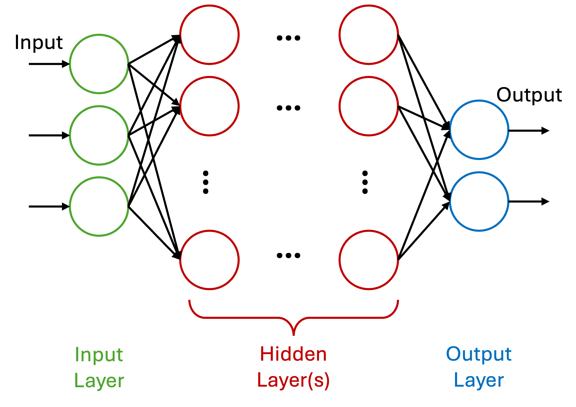
Figure 1 illustrates the overall architecture of an MLP, which typically includes one input layer, one or more hidden layers, and one output layer [2, 3].

• Input Layer: The number of neurons in the input layer corresponds to the number of features in the dataset.

• Hidden Layer: The network may include one or multiple hidden layers, each containing an arbitrary number of neurons. These layers are responsible for learning hierarchical feature representations.

• Output Layer: This layer generates the final prediction or output of the model.

Since neurons in an MLP are typically densely connected, most architectures are fully connected, i.e., each neuron in one layer is connected to all neurons in the subsequent layer [2, 3].

Mechanisms

Each MLP operates based on four fundamental mechanisms: forward propagation, loss computation, backpropagation, and optimization [2, 3].

Forward Propagation

During forward propagation, data flows from the input layer to the output layer, passing through the hidden layers. Each neuron processes the input in two steps [2, 3].

1. Weighted Sum: Each neuron computes a weighted sum of its inputs as [2, 3]

   \[ z = \sum_{i=1}^{N} w_{i}x_{i} + b, \]

   where \(N\) is the number of inputs, \(x_{i}\) represents the input data, \(w_{i}\) the corresponding weights, and \(b\) the bias term. This operation establishes a linear relationship among inputs, weights, and bias [2, 3].

2. Activation Function: To introduce non-linearity, an activation function is applied to \(z\). Common activation functions include [2, 3]:

   • Sigmoid:

     \[ \sigma(z) = \frac{1}{1 + e^{-z}} \]

   • Rectified Linear Unit (ReLU):

     \[ f(z) = \max\{0, z\} \]

   • Hyperbolic Tangent (Tanh):

     \[ \tanh(z) = \frac{2}{1 + e^{-2z}} - 1 \]

Loss Function

The loss function quantifies the difference between predicted and actual values, that guides the optimization process. Selecting an appropriate loss function is crucial for effective training. Common loss functions include [2, 3]:

• Binary Classification: Binary Cross-Entropy Loss (BCELoss) is suitable when the output layer contains a single neuron. For \(N\) samples, with true labels \(y_{i}\) and predicted probabilities \(\hat{y}_{i}\), the loss is defined as [2, 3]:

  \[ \mathcal{L} = -\frac{1}{N}\sum_{i=1}^{N}\left[ y_{i}\log(\hat{y}_{i}) + (1 - y_{i})\log(1 - \hat{y}_{i})\right] \]

• Multi-class Classification: For tasks with \(C\) classes, Cross-Entropy Loss (CELoss) is used. The output layer includes \(C\) neurons, each representing a class [2, 3]:

  \[ \mathcal{L} = -\frac{1}{N}\sum_{i=1}^{N}\sum_{c=1}^{C} y_{ic}\log(\hat{y}_{ic}) \]

• Regression: Mean Squared Error (MSE) Loss is commonly used for regression tasks [2, 3]:

  \[ \mathcal{L} = \frac{1}{N}\sum_{i=1}^{N}(y_{i} - \hat{y}_{i})^{2} \]

Backpropagation

The objective of training is to minimize the loss by updating the network's parameters (weights and biases). Backpropagation is the process through which this minimization is achieved [2, 3].

1. Gradient Calculation: In the backpropagation, the mode first computes the gradient of the loss function w.r.t. each weight and bias [2, 3].

2. Error Propagation: In this step, the computed errors are propagated backward from the output layer to the input layer [2, 3].

3. Parameter Update: Finally, weights and biases are updated using the gradient descent rule with a defined learning rate \(\alpha\) [2, 3]:

   \[ \begin{split} w &\leftarrow w - \alpha\frac{\partial\mathcal{L}}{\partial w},\\ b &\leftarrow b - \alpha\frac{\partial\mathcal{L}}{\partial b} \end{split} \]

Optimization

Optimization algorithms are applied to adjust the weights and biases efficiently based on the gradients. Two widely used optimization techniques in MLPs are Stochastic Gradient Descent (SGD) [4] and Adaptive Moment Estimation (Adam) [5].

• Stochastic Gradient Descent (SGD): In SGD, the model updates parameters using a single (or small batch of) training samples at each iteration, rather than the entire dataset. This approach improves computational efficiency and helps escape local minima. The parameter update rule is [4]:

  \[ \theta \leftarrow \theta - \alpha \nabla_{\theta}\mathcal{L}(\theta; x_{i}, y_{i}), \]

  where \(\alpha\) is the learning rate, \(\theta\) denotes model parameters, and \(\nabla_{\theta}\mathcal{L}\) represents the gradient of the loss [4].

• Adaptive Moment Estimation (Adam):: SGD is prone to trapping in local minima. To address this limitation, Adam combines the advantages of SGD with momentum and adaptive learning rates. It uses momentum to accelerate the gradient descent process by incorporating an exponentially weighted moving average of past gradients. This helps smooth out the trajectory of the optimization allowing the algorithm to converge faster by reducing oscillations. The update rule with momentum is given by [5]:

  \[ w_{t + 1} = w_{t} - \alpha m_{t}, \]

  where \(m_{t}\) is the moving average of the gradients at time \(t\); parameter \(\alpha\) shows the learning rate; and \(w_{t}\) and \(w_{t+1}\) represent the weights of the model at times \(t\) and \(t + 1\), respectively. The momentum term \(m_{t}\) is updated recursively as [5]

  \[ m_{t} = \beta_{1}m_{t - 1} + (1 - \beta_{1})\frac{\partial\mathcal{L}}{\partial w_{t}}, \]

  where \(\beta_{1}\) is the momentum parameter (typically set to 0.9), \(\partial\mathcal{L}/\partial w_{t}\) is the gradient of the loss function w.r.t. the weights at time \(t\) [5].

  Adam also exploits Root Mean Square Propagation (RMSprop) that helps overcome the problem of diminishing learning rates via exponentially weighted moving average of squared gradients. The update rule for RMSprop is [5]

  \[ w_{t + 1} = w_{t} - \frac{\alpha_{t}}{\sqrt{v_{t} + \epsilon}}\frac{\partial\mathcal{L}}{\partial w_{t}}, \]

  where \(\epsilon\) is a small constant to avoid division by zero. Also, \(v_{t}\) is the exponentially weighted average of squared gradients that is given by [5]

  \[ v_{t} = \beta_{2}v_{t - 1} + (1 - \beta_{2})\left(\frac{\partial\mathcal{L}}{\partial w_{t}}\right)^{2}, \]

  where \(\beta_{2}\) is the decay rate (typically set to 0.999) [5].

  Overall, Adam maintains exponentially decaying averages of past gradients (first moment) and squared gradients (second moment), allowing for stable and fast convergence. Its update rules are [5]:

  \[ \begin{split} \hat{m}_{t} &= \frac{m_{t}}{1 - \beta_{1}^{t}}, \quad \hat{v}_{t} = \frac{v_{t}}{1 - \beta_{2}^{t}} \\ \theta_{t} &= \theta_{t-1} - \alpha \frac{\hat{m}_{t}}{\sqrt{\hat{v}_{t}} + \epsilon}, \end{split} \]

Adam generally outperforms vanilla SGD in practice due to its adaptive learning rate and momentum terms, especially in high-dimensional and sparse datasets [5].

Implementation

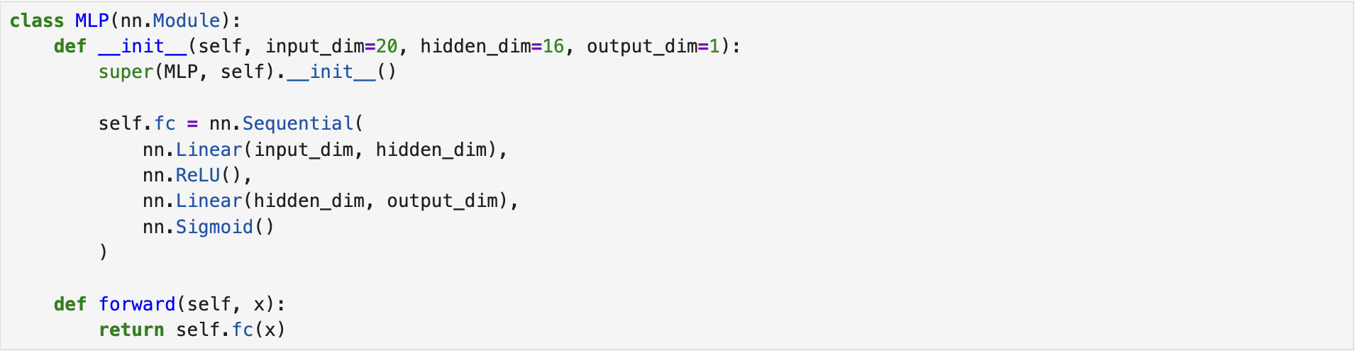
We developed two MLP networks for a binary classification task to demonstrate the difference between the Binary Cross-Entropy Loss (BCELoss) and the Cross-Entropy Loss (CELoss) functions. The models were implemented using the PyTorch [6] framework. Both MLPs consist of one input layer, one hidden layer, and one output layer. The input and hidden layers contain 20 (corresponding to the number of features) and 16 neurons, respectively. However, the output layers differ in the number of neurons depending on the selected loss function.

The first MLP uses BCELoss as its loss function. Therefore, the output layer consists of a single neuron with a Sigmoid activation function. The following screenshot illustrates the architecture of the corresponding MLP class.

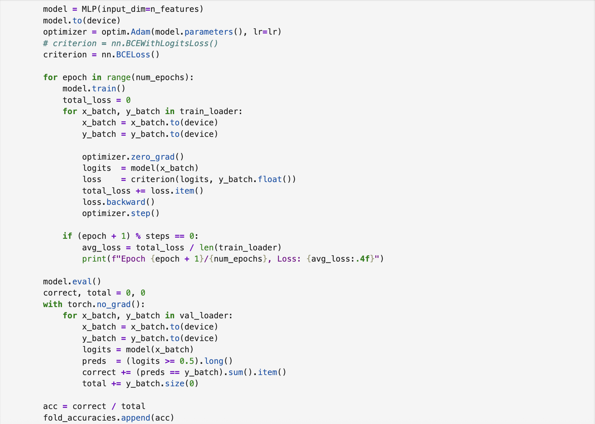
The training was conducted for 100 epochs, and k-fold cross-validation was applied to mitigate overfitting and improve model generalization. The following screenshot shows the training and validation procedures under k-fold cross-validation. The complete implementation script is available on BCELoss-based MLP.

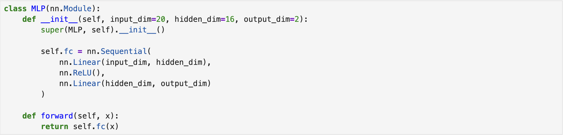
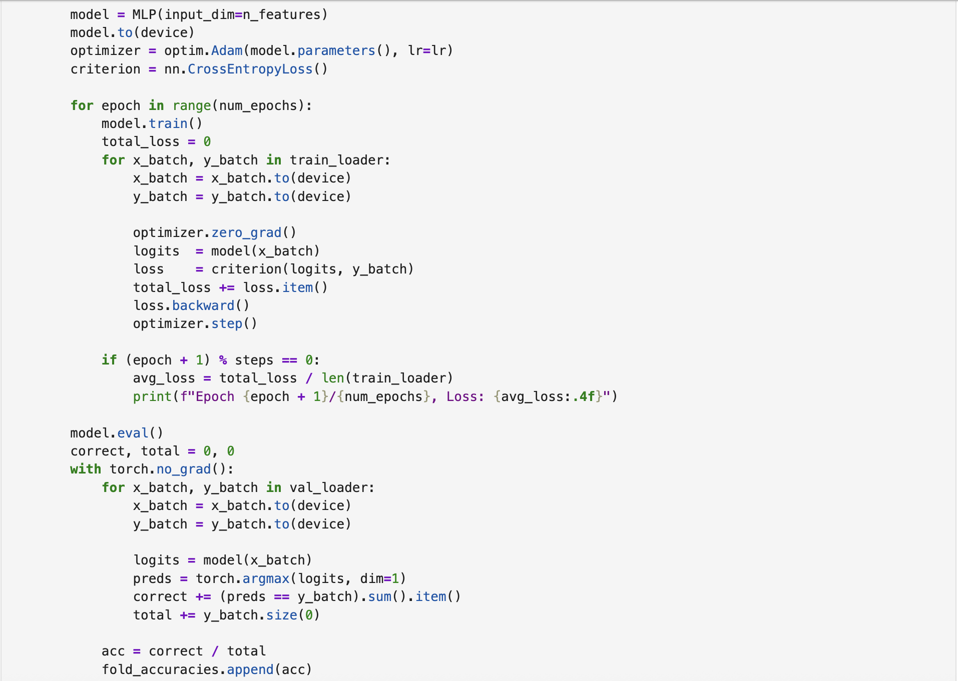
The second model leverages CELoss as the loss function. In this case, the output layer contains two neurons corresponding to the two classes. The following screenshot shows the corresponding MLP class defined for this model.

Similar to the BCELoss-based MLP, this model was trained for 100 epochs using k-fold cross-validation. The following screenshot presents the training and validation process. As shown, to obtain the corresponding label, argmax function is applied to the logits. The complete implementation script is available on CELoss-based MLP.

References

[1] F. Pedregosa, G. Varoquaux, A. Gramfort, V. Michel, B. Thirion, O. Grisel, M. Blondel, P. Prettenhofer, R. Weiss, V. Dubourg, J. Vanderplas, A. Passos, D. Cournapeau, M. Brucher, M. Perrot, and E. Duchesnay, “Scikit-learn: Machine learning in Python,” Journal of Machine Learning Research, vol. 12, pp. 2825–2830, 2011.

[2] GeeksforGeeks, “Multi-layer perceptron learning in tensorflow,” GeeksforGeeks, accessed: September 30, 2022, https://www.geeksforgeeks.org/deep-learning/multi-layer-perceptron-learning-in-tensorflow/.

[3] Adrian Tam, “Building Multilayer Perceptron Models in PyTorch,” Machine Learning Mastery, accessed: April 8, 2023, https://machinelearningmastery.com/building-multilayer-perceptron-models-in-pytorch/.

[4] GeeksforGeeks, “ML - Stochastic Gradient Descent (SGD),” GeeksforGeeks, accessed: September 30, 2025, https://www.geeksforgeeks.org/machine-learning/ml-stochastic-gradient-descent-sgd/.

[5] GeeksforGeeks, “What is Adam Optimizer?,” GeeksforGeeks, accessed: October 4, 2025, https://www.geeksforgeeks.org/deep-learning/adam-optimizer/.

[6] Adam Paszke et al., “PyTorch: An Imperative Style, High-Performance Deep Learning Library,”, 2019. https://arxiv.org/abs/1912.01703.