Convolutional Neural Network

Convolutional Neural Networks (CNNs) are inspired by the human visual system. The eyes serve as input gates that capture visual information and transmit it to the brain, where the visual cortex processes the image step by step (layer by layer) to recognize the components of the scene.

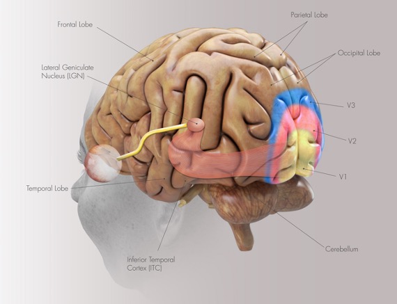
Fig. 1: Visual cortex in the human brain [1].

Figure 1 shows the visual cortex in the human brain, including the Retina, Lateral Geniculate Nucleus (LGN), Primary Visual Cortex (V1), Secondary Visual Cortex (V2), Tertiary Visual Cortex (V3), and Lateral Occipital Complex (LOC) [1].

Retina: A layer of photoreceptors at the back of the eye that detects light intensity and color (wavelength). The retina converts optical images into electrical signals and sends them via the optic nerve to the LGN [1].
Lateral Geniculate Nucleus (LGN): Acts as a relay station between the retina and V1. It organizes, filters, and modulates visual signals while maintaining spatial mapping of the visual scene, a property known as retinotopy [1].
Primary Visual Cortex (V1): Processes basic features such as edge orientation, contrast, and motion direction. Neurons in V1 have receptive fields that respond to stimuli in specific locations of the visual field [1].
Secondary Visual Cortex (V2): Combines information from V1 to process more complex patterns, including contours, textures, and simple shapes. V2 serves as an intermediate stage that prepares visual information for higher-level processing [1].
Tertiary Visual Cortex (V3): Divided into two parts [1]:
- V3 proper (dorsal V3): Involved in motion and dynamic form processing. It is part of the dorsal stream (“where/how” pathway) that extends toward the parietal lobe, responsible for motion, depth, and spatial awareness [1].
- V3v (ventral V3): Involved in object shape and form processing. It is part of the ventral stream (“what” pathway) that extends toward the inferotemporal cortex (IT) and is responsible for object recognition, color, and detailed form [1].
Lateral Occipital Complex (LOC): Recognizes c omplete objects, responding to shapes and forms regardless of size, position, or viewpoint [1].

Inspired by this biological system, a CNN combines convolutional layers with a fully connected neural network. Figure 2 illustrates a typical CNN architecture including two convolutional layers followed by a fully connected MLP. The model is trained on the MNIST dataset and classifies each input image into one of ten classes (digits 0–9).

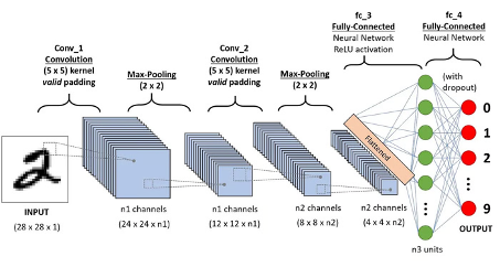
Fig. 2: An example architecture of a CNN [2].

A convolutional layer in a CNN consists of number of channels (e.g., \(n_{1}\) and \(n_{2}\) in Fig. 2), each equipped with a fundamental building block called a kernel or filter. Filters in each layer learn to recognize patterns, progressively identifying more complex features in deeper layers. Figure 3 illustrates this hierarchical learning process.

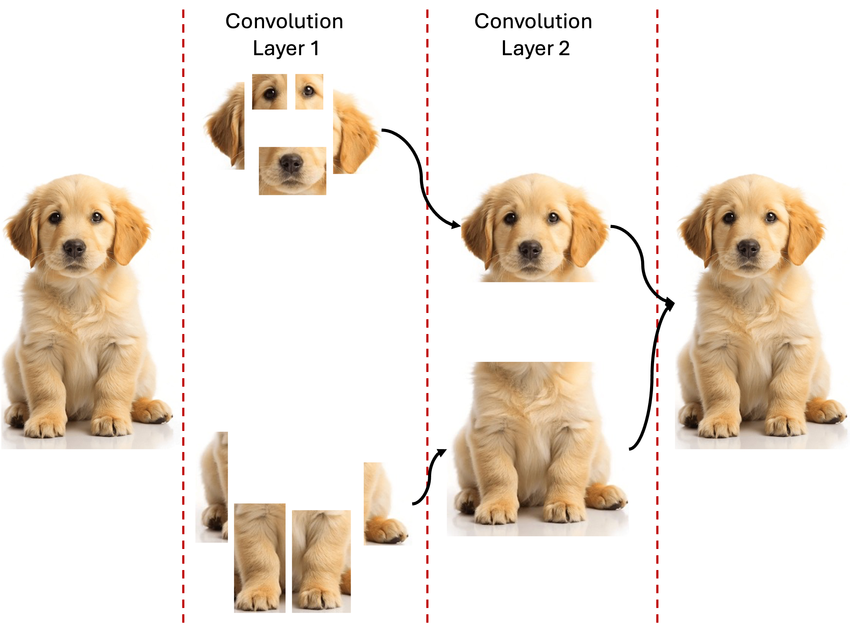
Fig. 3: An example of convolutional layers in a CNN.

In this example, an initial image (a cute dog; image source: Pinterest [3]) is filtered by kernels in the first convolutional layer. The upper filters learn to detect features such as eyes, nose, and ears, while the lower filters recognize paws. In the second layer, the filters identify higher-level structures such as the head and body. This hierarchical learning enables CNNs to build complex visual understanding from simple features.

In the following subsections, we review the core components of a CNN, followed by implementing a CNN model.

Filter

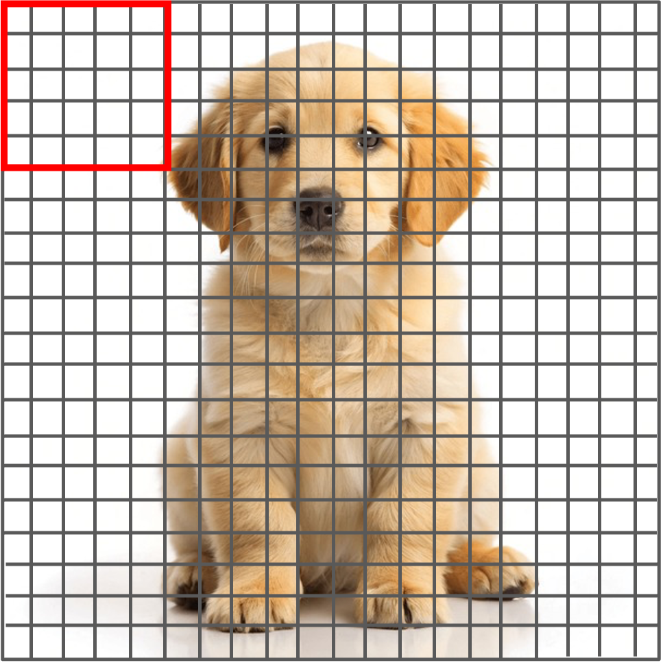
A filter (or kernel) in a CNN detects local patterns in an image. Given an input image of size \((n \times n)\), a filter of size \((f \times f)\) slides over the image, performing element-wise multiplications and summations with corresponding pixel values. The result at each step forms the corresponding pixels in the output feature map [2]. Figure 4 shows an example of a \((20 \times 20)\) input image with a \((5 \times 5)\) filter.

Fig. 4: Filter operation in a CNN.

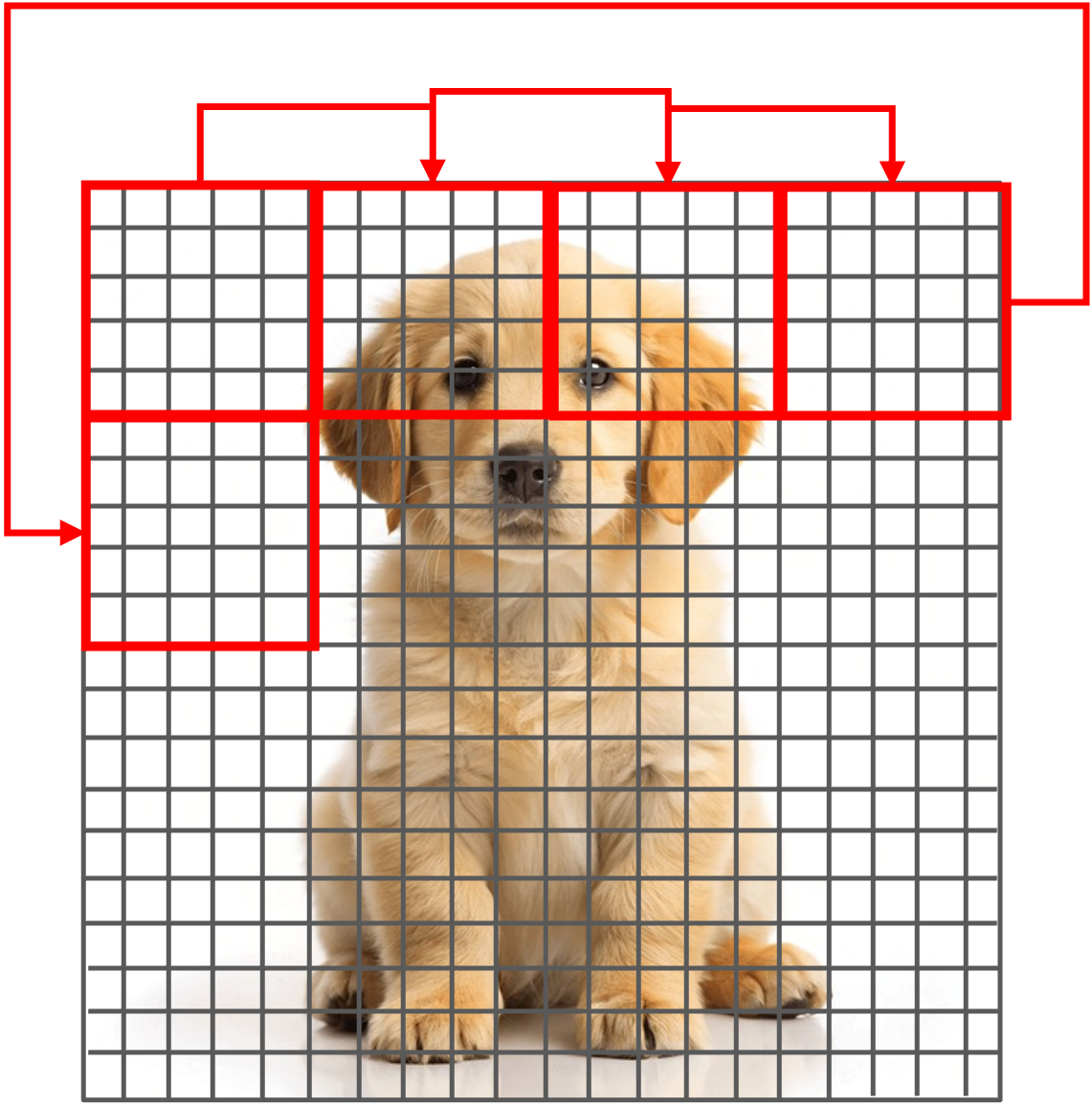
Stride

The stride determines how many pixels the filter moves each time it slides over the input image [2]. Figure 5 shows an example where the stride is \((5, 5)\), stating that the filter moves five pixels to the right after each operation and, upon reaching the end of a row, moves five pixels down to start the next pass.

Fig. 5: Stride in a CNN.

Padding

Padding controls the spatial dimensions of the output feature maps. Without padding, applying filters reduces the size of the feature maps. To preserve the input dimensions, zeros are added around the borders of the input image. Given an input of size \((n \times n)\), filter size \((f \times f)\), and stride \(s\), the output dimension is calculated as [2]

\[ \text{output_size} = \left(\frac{n - f}{s} + 1 \right)\times \left(\frac{n - f}{s} + 1 \right) \]

In our example (Fig. 4), the output size is \((4 \times 4)\). There are two common types of padding:

Valid No padding is applied; thus, \(n' = n\), where \(n'\) is the new size of the input image [2].
Same Padding is applied such that the output size equals the input size. Let \(p\) be the padding size. Since padding happens for rows (up and down) and columns (left and right), the new input images size must follow \(n' = n + 2p\). Therefore, we have [2].

\[ \frac{n' - f}{s} + 1 = n \Rightarrow \frac{n + 2p - f}{s} + 1 = n \Rightarrow p = \frac{n(s - 1) + f - s}{2} \]

Figure 6 illustrates zero-padding (or Same) in an input image.

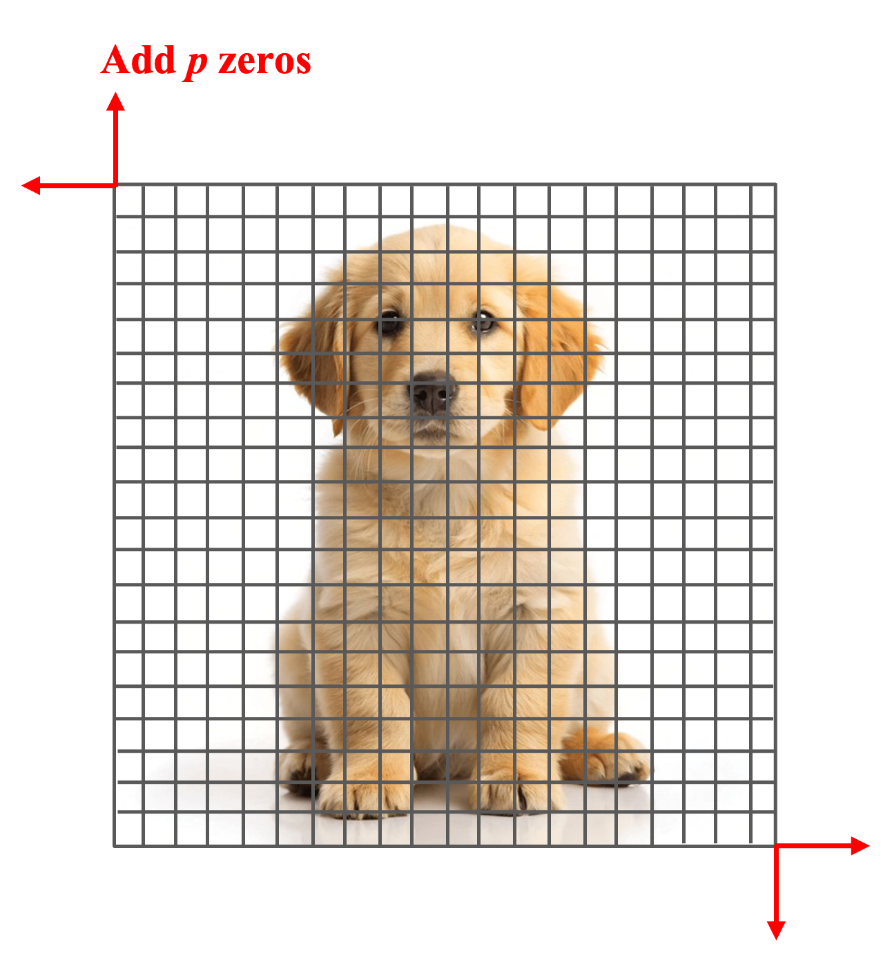
Fig. 6: Padding in a CNN.

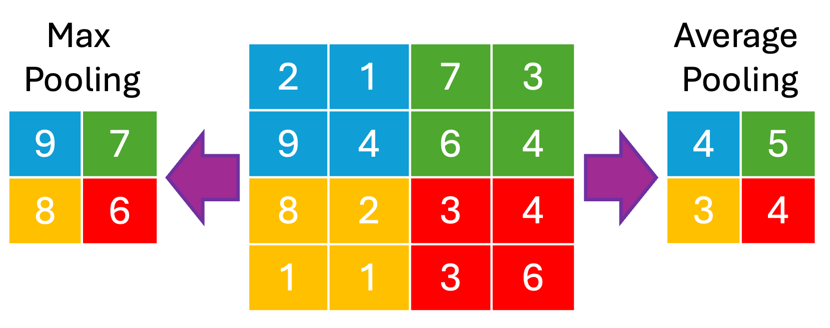
Pooling

Pooling is a downsampling technique used to reduce the spatial size of feature maps, which decreases computational cost and helps prevent overfitting by summarizing local features. The two most common pooling methods are Max Pooling and Average Pooling, which select the maximum or average value from each region, respectively [2]. Figure 7 shows an example using a \((2 \times 2)\) filter and a \((2, 2)\) stride.

Fig. 7: Pooling in a CNN. Left: Max Pooling; Right: Average Pooling.

Fully Connected Neural Network

The final stage of a CNN is a fully connected neural network (an MLP) that maps the extracted features to output predictions (e.g., class probabilities). The output of the convolutional layers is first flattened into a one-dimensional vector and then passed through one or more dense layers to produce the final outputs [2].

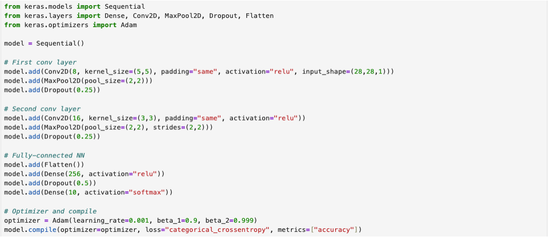
Implementation

The following screenshot illustrates the training process of a CNN model implemented in the TensorFlow [4] framework. The complete implementation script is available on CNN.

References

[1] Ophthalmology Training.com, “Visual Cortex,” Ophthalmology Training.com, accessed: 2022, https://www.ophthalmologytraining.com/core-principles/ocular-anatomy/visual-pathway/visual-cortex.

[2] Zoumana Keita, “An Introduction to Convolutional Neural Networks (CNNs),” Datacamp, accessed: November 14, 2023, https://www.datacamp.com/tutorial/introduction-to-convolutional-neural-networks-cnns.

[3] Pinterest, https://www.pinterest.com/.

[4] Martin Abadi et al., “TensorFlow: Large-Scale Machine Learning on Heterogeneous Systems,” Software available from tensorflow.org, accessed: 2015, https://www.tensorflow.org/.

Forough Shirin Abkenar