Encoder-only Models

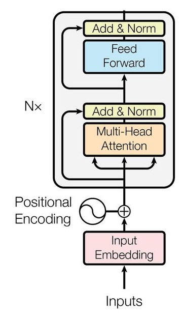
The encoder-only models in LLMs owns the LLM architecture with only the encoder transformer (see the following Fig. 1). The encoder in the LLM architecture is responsible for receiving the input data (prompts) and embedding (encoding) them into meaningful output (vector representation). Encoder-only models exploit bidirectional processing of data whereby the input tokens are processed using information from both left and right to understand the token's context.

Bidirectional encoder representations from transformers (BERT) [2] and robustly optimized BERT pretraining approach (RoBERTa) [3] models are types of encoder-only models that are applicable for text classification, sentiment analysis, named entity recognition (NER), and etc.

As seen in Fig. 1, the inputs in the encoder-only model are passed through sequential components, i.e., input embedding, positional encoding, and encoder layer (shown as Nx in the figure). In the rest of the current chapter, we review each layer and the corresponding mechanisms.

Input Embedding

In encoder-only models, the inputs are textual data, represented as sequences of text units such as words, subwords, or characters. However, the encoder block processes numerical representations rather than raw text. To bridge this gap, an input embedding layer converts textual inputs into numerical IDs. This process relies on a predefined vocabulary in which each text unit, commonly referred to as a token, is mapped to a unique identifier, namely token ID. Notably, each token ID is a vector of numbers with a shape of prdefined embedding dimensiion. Consequently, the input text undergoes tokenization, where it is divided into tokens, and then each token is mapped to the corresponding token ID.

Positional Encoding

Positional encoding is a mechanism whereby the information about the position of a token is injected to the input data. Hence, the model can learn the meaning and importance of the corresponding token w.r.t. its position in the input (subject, object, verb, adjective, etc.). The traditional positional encoding is calculated using the sin and cos equations in [1].

Encoder Layer

The encoder layer (shown Nx in Fig. 1) comprises two sub-layers. The first sub-layer implements the multi-head self-attention mechanism, and the second sub-layer is a fully-connected feed-forward neural network. Each sub-layer has a residual connection around itself, and also is succeeded by a normalization layer [1].

Multi-Head Self-Attention Mechanism

The self-attention mechanism is a core component of transformers, enabling the model to learn and capture the relationships between tokens within a sequence. This mechanism is implemented within the attention heads of the transformer architecture [1].

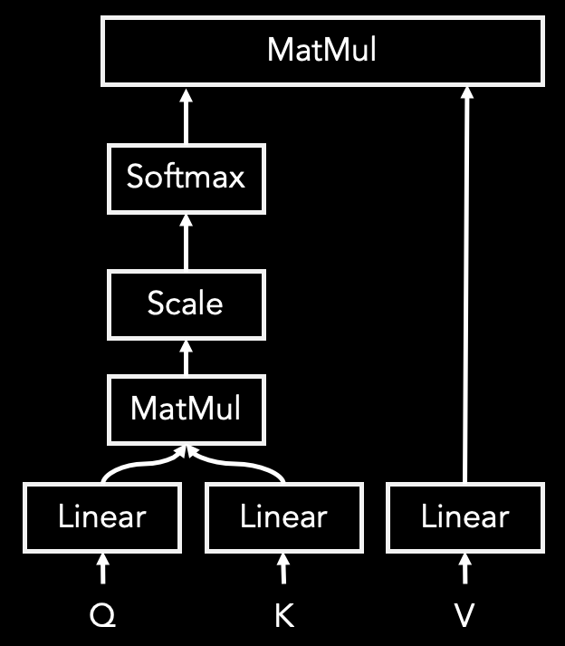
To model the relationships between tokens, the input is first projected into three distinct representations: the query (Q), key (K), and value (V) vectors. Figure 2 illustrates the architecture of an attention head within the model. When an embedded and positionally encoded input passes through the attention head, it undergoes the following five processing steps [1]:

• Step 1: query (Q), key (K), and value (V) components are passed through linear layers in the attention head model so that these components are learned.

• Step 2: the alignment scores are calculated through multiplication of matrices query and key.

• Step 3: the alignment scores are scaled by 1/d_k, where d_k is the dimension of the query (or the key) matrix.

• Step 4: softmax operation is applied to the scaled scores to obtain the attention weights.

• Step 5: the attention weights are multiplied with the value matrix.

The multi-head self-attention mechanism consists of multiple parallel attention heads, each learning distinct representation subspaces. The outputs from all attention heads are concatenated and then projected through a linear layer to produce the final combined representation [1].

Add & Norm

Residual Connections (Add): Preserving information from earlier layers helps mitigate the vanishing gradient problem. In transformer encoders, this is achieved through residual connections, where the original input of a layer is added to its output. This mechanism enables the network to retain essential information across layers and facilitates more effective gradient flow during training [1].

Layer Normalization (Norm): During training, the model may experience internal covariate shift, where the distribution of activations changes across layers, potentially leading to vanishing or exploding gradients. To address this challenge, layer normalization is applied to the outputs of deeper layers that in result, stabilizes training by reducing distributional shifts and ensures more consistent gradient flow [1].

Feed-Forward Network

The feed-forward sub-layer introduces non-linearities into the encoder, thereby enhancing the model's capacity to capture complex patterns and non-linear relationships within sequential data. The feed forward network consists of two linear transformations separated by an activation function, typically the rectified linear unit (ReLU) or the Gaussian error linear unit (GELU) [1].

Implementation

In this section, we use a small input text to develop a minimal encoder-only model, called TinyBert. The goal is to gain familiarity with the operation of encoder-only models. The overall network architecture is shown below, and the complete implementation script is available on Encoder-only.

As defined in the __init__ function, the model network includes the following layers:

• self.token_embed: it creates an embedding layer that converts token indices (integers) into dense vector representations (embeddings).

• self.pos_embed: this layer create the positional encoding of the input tokens.

• self.blocks: it includes encoder blocks (layers), each with a multi-head self-attention head, a feed forward network, and the corresponding add & norm components.

• self.ln_f: this layer defines the final layer normalization applied to the transformer's output before passing it into the language modeling head.

• self.mlm_head: it defines the masked language model (MLM) head, i.e., the final layer that maps the hidden representations produced by the transformer into predicted token probabilities.

When an input passes through the forward function, it is first converted into token embeddings. Positional embeddings are then added to incorporate information about token order. The resulting representations are sequentially passed through all the transformer blocks defined in the model. The output of the final block is normalized using the last layer normalization and then fed into the language modeling head. At this stage, each token is represented by a hidden vector of size equal to the embedding dimension, and the final layer predicts the probability distribution over the vocabulary for the next token.

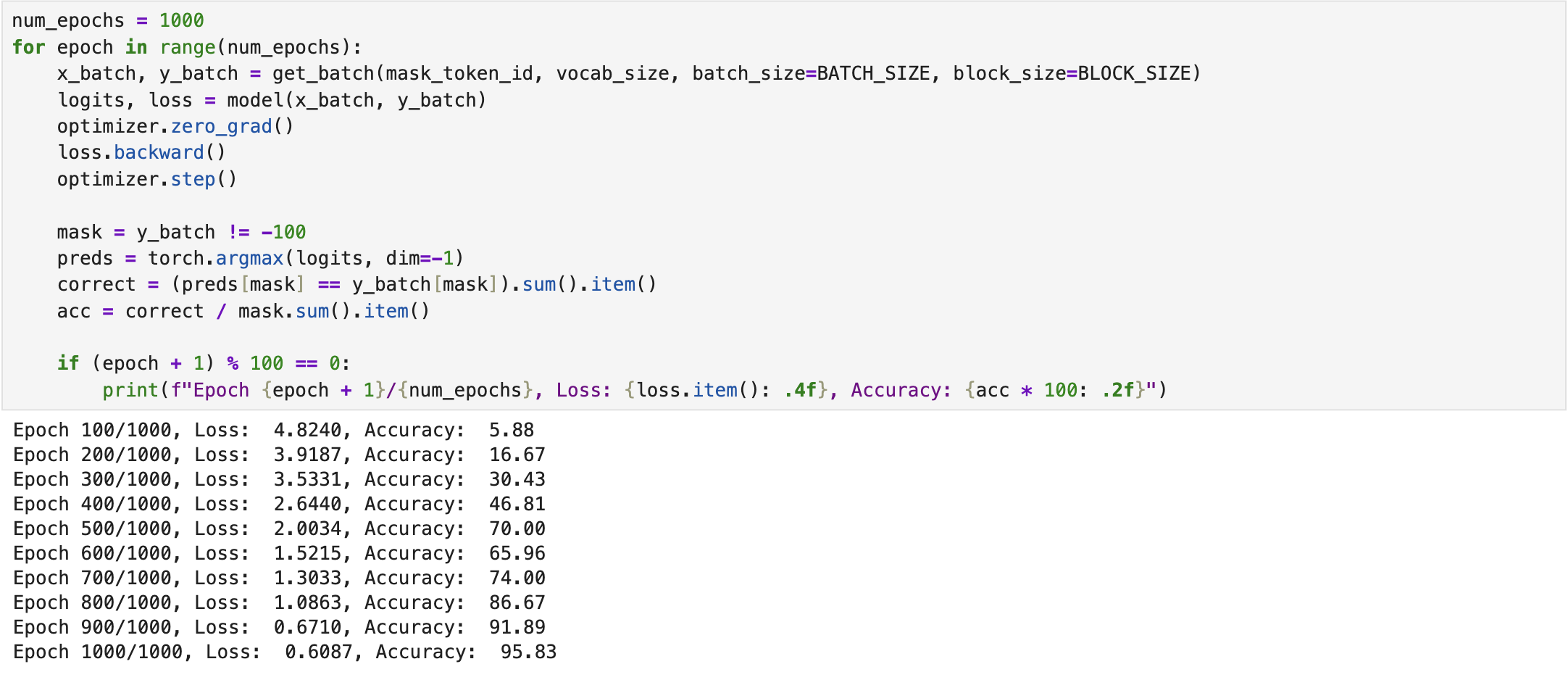
During training, the model compares these predicted logits with the true token IDs using cross-entropy loss, and updates its weights through backpropagation to minimize this loss.

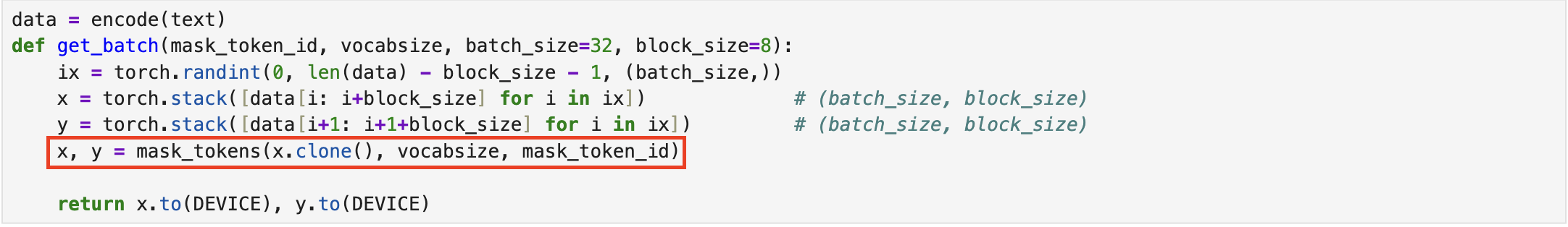
Since the primary objective of the designed TinyBert model is to predict masked tokens in the input text, the get_batch function used during training incorporates a mask_token function based on the MLM strategy. This function applies an 80/10/10 masking rule: 80% of tokens are replaced with a predefined mask token (e.g., “[MASK]”), 10% are substituted with random tokens from the vocabulary, and the remaining 10% are left unchanged.

Evaluation

For evaluation, we select a portion of the text, mask certain words, and assess the model's performance in predicting these masked tokens. Accordingly, we compute the cross-entropy loss, perplexity, and accuracy on the masked words: (1) cross-entropy loss measures the difference between the predicted probability distribution of a model and the true distribution of the target data; lower values indicates better predictions and less uncertainty. (2) perplexity measures the model's uncertainty; lower perplexity implies that the model assigns higher probability to the actual next word in the sequence, resulting a more confident and accurate model. (3) accuracy measures how well the model predicts the masked tokens, with higher values indicating more correct predictions. Table I indicates the performance of TinyBert w.r.t. the aforementioned evaluation metrics.

References

[1] A. Vaswani, N. Shazeer, N. Parmar, J. Uszkoreit, L. Jones, A. N. Gomez, L. Kaiser, and I. Polosukhin, “Attention is all you need,” Advances in Neural Information Processing Systems, vol. 30, 2017, https://arxiv.org/abs/1706.03762.

[2] J. Devlin, M.-W. Chang, K. Lee, and K. Toutanova, “Bert: Pre-training of deep bidirectional transformers for language understanding,” in North American Chapter of the Association for Computational Linguistics, 2019, https://api.semanticscholar.org/CorpusID:52967399.

[3] Y. Liu, M. Ott, N. Goyal, J. Du, M. Joshi, D. Chen, O. Levy, M. Lewis, L. Zettlemoyer, and V. Stoyanov, “Roberta: A robustly optimized bert pretraining approach,” ArXiv, vol. abs/1907.11692, 2019, https://api.semanticscholar.org/CorpusID:198953378.